#!/usr/bin/env python
# coding: utf-8
# # Nonlinear equations II
# In[ ]:
# ## Outline
# * Fixed point iteration
# * Secant method
# * Newton's method
#
# ## Comments
# * Focusing on 1 equation and 1 unknown here.
# * Methods only require information at one point.
# * Termed "open" methods
# * Unlike the closed (bracketing) methods that required two initial points.
# * Methods may converge faster.
# * Methods may diverge (the tradeoff).
# * Often used to refine a root from a slower method like bisection.
# ## Fixed point method
# * Very common
# * Very simple
# * Rewrite $f(x)=0$ as $x=g(x)$.
# * Can always do this: just add $x$ to both sides.
# * But there is often more than one way to do this, and the approch used may affect stability, as shown below.
# * Iteration:
# $$x_{k+1} = g(x_k)$$
# * That is: guess $x_0$.
# * Evaluate $g(x_0)$.
# * The result is $x_1$.
# * Repeat.
#
# Geometrically $x_{k+1} = g(x_k)$ finds the intersection of the $y=g(x)$ and $y=x$ lines.
#
# 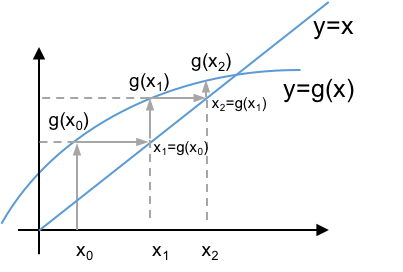 #
# * Convergence depends on:
# 1. Initial guess
# 2. Form chosen for $g(x)$.
#
# * **Example**
# $$ f(x) = x^2-x-2$$
# * Roots at $x=2$, $x=-1$.
# * Several forms, different behavior:
# * Add $x$ to both sides of $f(x)=0$: $$x = x^2-2 = g(x).$$
# * Add $x+2$ to both sides of $f(x)=0$, and divide the result by $x$: $$x=1+\frac{2}{x} = g(x).$$
# * Add $x+2$ to both sides and then take the square root: $$x = \sqrt{x+2} = g(x).$$
# * Add $x^2+2$ then divide by $(2x-1)$: $$x = \frac{x^2+2}{2x-1} = g(x).$$
# In[1]:
import numpy as np
import matplotlib.pyplot as plt
get_ipython().run_line_magic('matplotlib', 'inline')
x = np.linspace(-2,3,100)
y1 = x**2 - 2.0
y2 = 1.0+2./x
y3 = (x+2.)**0.5
y4 = (x**2 + 2)/(2*x -1)
plt.rc("font", size=16)
plt.plot(x,y1,label=r'$x^2-2$')
plt.plot(x,y2,label=r'$1+2/x$')
plt.plot(x,y3,label=r'$(x+2)^{1/2}$')
plt.plot(x,y4,label=r'$(x^2+2)/(2x-1)$')
plt.plot(x,x,'k--',label=r'$x$')
plt.legend(loc='upper left', frameon=False, fontsize=12)
plt.ylim([-1,8]); # plt.ylim([-3,8])
plt.xlim([1,3]); # plt.xlim([-2,3])
plt.xlabel('x')
plt.ylabel('g(x)');
# ### Fixed point example 1
# * Solve $x=g(x)$ for $g(x) = (x+2)^{1/2}$.
# In[2]:
import numpy as np
def FP(g, x, tol=1E-5, maxit=1000):
for niters in range(1,maxit+1):
xnew = g(x)
err = np.linalg.norm(xnew-x)/np.linalg.norm(x)
if err <= tol:
return xnew, niters
x = xnew
print(f"Warning no converged in {maxit} iterations")
return xnew, niters
# In[15]:
def FP(g, x, tol=1E-5, maxit=1000):
for niter in range(1,maxit+1):
xnew = g(x)
if np.linalg.norm(xnew-x)/np.linalg.norm(x) <=tol:
return xnew, niter
x = xnew
print('warning, reached maxit =', maxit)
return x, niter
#-----------
def g(x):
return np.sqrt(x+2)
#-----------
xguess = 4.0
x, nit = FP(g, xguess)
print("x, nit = ", x, nit)
# ## Fixed point example 2
# * Fluid mechanics, turbulent pipe flow
# * Given $\Delta P$, $D$, $L$, $\epsilon/D$, $\rho$, $\mu$.
# * Find the velocity in the pipe.
#
# Equations:
#
# $$ Re = \frac{\rho Dv}{\mu}.$$
#
# $$ \frac{1}{\sqrt{f}} = -\log_{10}\left(\frac{\epsilon/D}{3.7} + \frac{2.51}{Re\sqrt{f}}\right),$$
#
# $$ \frac{\Delta P}{\rho} = \frac{fLv^2}{2D} \rightarrow v = \sqrt{\frac{2D\Delta P}{\rho f L}}.$$
# Approach:
# * Let unknowns be $v$ and $\hat{f}\equiv 1/\sqrt{f}$.
# * Guess $v_0$ and $\hat{f}_0$
# * Solve for $Re$ from the first equation above.
# * Solve for $\hat{f}$
# * Solve the third equation above for $v$.
# * Repeat.
#
# Note, this calls ```FP``` from example 1
# In[16]:
import numpy as np
#-------------------
def g_fluids(vfhat):
v = vfhat[0]
fhat = vfhat[1]
ρ = 1000 # kg/m3
μ = 1E-3 # Pa*s = kg/m*s
D = 0.1 # m
L = 100 # m
ϵ = D/100 # m
ΔP = 101325 # Pa
Re = ρ*D*v/μ
fhat = -np.log10(ϵ/D/3.7 + 2.51*fhat/Re)
v = np.sqrt(2*D*ΔP/ρ/L)*fhat
return np.array([v, fhat])
#-------------------
vfhat_g = np.array([1.0, 0.1])
vfhat, nit = FP(g_fluids, vfhat_g)
print(f"v = {vfhat[0]:.4f} (m/s)")
print(f"f = {1/vfhat[1]**2:.4f}")
print(f"# iterations = {nit}")
# ### Convergence
# * For convergence, need the $|\mbox{slope}|<1.$
# * $x_{k+1} = g(x_k)$
# * At convergence, we have $x=g(x)$.
# * Subtract these two: $x_{k+1}-x = \epsilon_{k+1} = g(x_k)-g(x)$
# * Now, expand g as a Taylor series: $g(x) = g(x_k) + g^{\prime}(\xi)(x-x_k)$, where $x\le\xi\le x_k$
# * Hence, $\epsilon_{k+1} = -g^{\prime}(\xi)(x-x_k) = g^{\prime}(\xi)\epsilon_k$
# * So, $$\frac{\epsilon_{k+1}}{\epsilon_k} = g^{\prime}(\xi).$$
# * For convergence, we need $$\left|\frac{\epsilon_{k+1}}{\epsilon_k}\right| = |g^{\prime}(\xi)| < 1.$$
# * At the solution, $|g^{\prime}(x)|<1$.
#
#
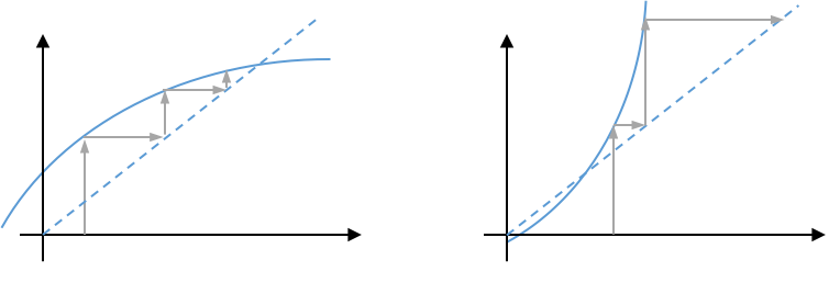
# * The plot on the left, below, converges, while the plot on the right diverges away from the solution.
#
#
# * Convergence depends on:
# 1. Initial guess
# 2. Form chosen for $g(x)$.
#
# * **Example**
# $$ f(x) = x^2-x-2$$
# * Roots at $x=2$, $x=-1$.
# * Several forms, different behavior:
# * Add $x$ to both sides of $f(x)=0$: $$x = x^2-2 = g(x).$$
# * Add $x+2$ to both sides of $f(x)=0$, and divide the result by $x$: $$x=1+\frac{2}{x} = g(x).$$
# * Add $x+2$ to both sides and then take the square root: $$x = \sqrt{x+2} = g(x).$$
# * Add $x^2+2$ then divide by $(2x-1)$: $$x = \frac{x^2+2}{2x-1} = g(x).$$
# In[1]:
import numpy as np
import matplotlib.pyplot as plt
get_ipython().run_line_magic('matplotlib', 'inline')
x = np.linspace(-2,3,100)
y1 = x**2 - 2.0
y2 = 1.0+2./x
y3 = (x+2.)**0.5
y4 = (x**2 + 2)/(2*x -1)
plt.rc("font", size=16)
plt.plot(x,y1,label=r'$x^2-2$')
plt.plot(x,y2,label=r'$1+2/x$')
plt.plot(x,y3,label=r'$(x+2)^{1/2}$')
plt.plot(x,y4,label=r'$(x^2+2)/(2x-1)$')
plt.plot(x,x,'k--',label=r'$x$')
plt.legend(loc='upper left', frameon=False, fontsize=12)
plt.ylim([-1,8]); # plt.ylim([-3,8])
plt.xlim([1,3]); # plt.xlim([-2,3])
plt.xlabel('x')
plt.ylabel('g(x)');
# ### Fixed point example 1
# * Solve $x=g(x)$ for $g(x) = (x+2)^{1/2}$.
# In[2]:
import numpy as np
def FP(g, x, tol=1E-5, maxit=1000):
for niters in range(1,maxit+1):
xnew = g(x)
err = np.linalg.norm(xnew-x)/np.linalg.norm(x)
if err <= tol:
return xnew, niters
x = xnew
print(f"Warning no converged in {maxit} iterations")
return xnew, niters
# In[15]:
def FP(g, x, tol=1E-5, maxit=1000):
for niter in range(1,maxit+1):
xnew = g(x)
if np.linalg.norm(xnew-x)/np.linalg.norm(x) <=tol:
return xnew, niter
x = xnew
print('warning, reached maxit =', maxit)
return x, niter
#-----------
def g(x):
return np.sqrt(x+2)
#-----------
xguess = 4.0
x, nit = FP(g, xguess)
print("x, nit = ", x, nit)
# ## Fixed point example 2
# * Fluid mechanics, turbulent pipe flow
# * Given $\Delta P$, $D$, $L$, $\epsilon/D$, $\rho$, $\mu$.
# * Find the velocity in the pipe.
#
# Equations:
#
# $$ Re = \frac{\rho Dv}{\mu}.$$
#
# $$ \frac{1}{\sqrt{f}} = -\log_{10}\left(\frac{\epsilon/D}{3.7} + \frac{2.51}{Re\sqrt{f}}\right),$$
#
# $$ \frac{\Delta P}{\rho} = \frac{fLv^2}{2D} \rightarrow v = \sqrt{\frac{2D\Delta P}{\rho f L}}.$$
# Approach:
# * Let unknowns be $v$ and $\hat{f}\equiv 1/\sqrt{f}$.
# * Guess $v_0$ and $\hat{f}_0$
# * Solve for $Re$ from the first equation above.
# * Solve for $\hat{f}$
# * Solve the third equation above for $v$.
# * Repeat.
#
# Note, this calls ```FP``` from example 1
# In[16]:
import numpy as np
#-------------------
def g_fluids(vfhat):
v = vfhat[0]
fhat = vfhat[1]
ρ = 1000 # kg/m3
μ = 1E-3 # Pa*s = kg/m*s
D = 0.1 # m
L = 100 # m
ϵ = D/100 # m
ΔP = 101325 # Pa
Re = ρ*D*v/μ
fhat = -np.log10(ϵ/D/3.7 + 2.51*fhat/Re)
v = np.sqrt(2*D*ΔP/ρ/L)*fhat
return np.array([v, fhat])
#-------------------
vfhat_g = np.array([1.0, 0.1])
vfhat, nit = FP(g_fluids, vfhat_g)
print(f"v = {vfhat[0]:.4f} (m/s)")
print(f"f = {1/vfhat[1]**2:.4f}")
print(f"# iterations = {nit}")
# ### Convergence
# * For convergence, need the $|\mbox{slope}|<1.$
# * $x_{k+1} = g(x_k)$
# * At convergence, we have $x=g(x)$.
# * Subtract these two: $x_{k+1}-x = \epsilon_{k+1} = g(x_k)-g(x)$
# * Now, expand g as a Taylor series: $g(x) = g(x_k) + g^{\prime}(\xi)(x-x_k)$, where $x\le\xi\le x_k$
# * Hence, $\epsilon_{k+1} = -g^{\prime}(\xi)(x-x_k) = g^{\prime}(\xi)\epsilon_k$
# * So, $$\frac{\epsilon_{k+1}}{\epsilon_k} = g^{\prime}(\xi).$$
# * For convergence, we need $$\left|\frac{\epsilon_{k+1}}{\epsilon_k}\right| = |g^{\prime}(\xi)| < 1.$$
# * At the solution, $|g^{\prime}(x)|<1$.
#
#
# * The plot on the left, below, converges, while the plot on the right diverges away from the solution.
#  #
# ## Secant method
# * Like Regula Falsi, but always use the last two points.
#
# $$x_{k+1} = x_k - \frac{f(x_i)}{\hat{f}^{\prime}_k},$$
#
#
#
# $$\phantom{xxxxxxxxxxxxxxx}\hat{f}_k = \frac{f(x_k)-f(x_{k-1})}{x_k-x_{k-1}}.$$
#
#
# * Here, $\hat{f}_k$ is the slope of $f$ at iteration $k$ based on the last two iteration points.
# * Might not bracket the root.
# * But much faster convergence.
# * This is an alternative to Newton's method (below), when we don't know or don't want to compute $f^{\prime}(x)$.
# * Requires two starting points.
#
# ### Convergence:
# * $\epsilon_{k+1} \propto \epsilon_k^{1.62}$.
# * *(Compare to fixed point method, where $\epsilon_{k+1} \propto \epsilon_k$.)*
# * Numerical Recipes says that this is more efficient than Newton's method if the cost of evaluating $f^{\prime}(x)<$ 43% of evaluating $f(x)$.
#
#
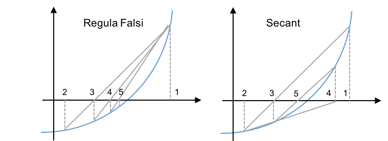
# ### Compare Secant and Regula Falsi methods:
#
#
# ## Secant method
# * Like Regula Falsi, but always use the last two points.
#
# $$x_{k+1} = x_k - \frac{f(x_i)}{\hat{f}^{\prime}_k},$$
#
#
#
# $$\phantom{xxxxxxxxxxxxxxx}\hat{f}_k = \frac{f(x_k)-f(x_{k-1})}{x_k-x_{k-1}}.$$
#
#
# * Here, $\hat{f}_k$ is the slope of $f$ at iteration $k$ based on the last two iteration points.
# * Might not bracket the root.
# * But much faster convergence.
# * This is an alternative to Newton's method (below), when we don't know or don't want to compute $f^{\prime}(x)$.
# * Requires two starting points.
#
# ### Convergence:
# * $\epsilon_{k+1} \propto \epsilon_k^{1.62}$.
# * *(Compare to fixed point method, where $\epsilon_{k+1} \propto \epsilon_k$.)*
# * Numerical Recipes says that this is more efficient than Newton's method if the cost of evaluating $f^{\prime}(x)<$ 43% of evaluating $f(x)$.
#
#
# ### Compare Secant and Regula Falsi methods:
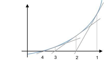
#  # ## Newton's method
# * Very popular
# * Extends easily to multiple dimensions
# * Quadratic convergence $\epsilon_{k+1} \propto \epsilon_k^2$.
# * Approach:
# * Approximate the function as linear at the current value of $x_k$.
# * Solve this linear equation for $x_{k+1}$.
# * This $x_{k+1}$ won't be the real answer because the real function is not linear. But $x_{k+1}$ will be an improvement.
# * Repeat the process at the new value of $x_{k+1}$.
#
# * Linearize the function using a Taylor series:
# $$f(x_{k+1}) = f(x_k) + f^{\prime}(x_k)(x_{k+1}-x_k)+(\ldots)$$
# * Ignore terms $(\ldots)$. Also, set $f(x_{k+1})=0$ and solve for $x_{k+1}$:
#
# $$ x_{k+1} = x_k - \frac{f(x_k)}{f^{\prime}(x_k)}.$$
#
# * This is like the Secant method, but instead of $\hat{f}^\prime_k$ we use $f^{\prime}(x_k)$.
#
# ## Newton's method
# * Very popular
# * Extends easily to multiple dimensions
# * Quadratic convergence $\epsilon_{k+1} \propto \epsilon_k^2$.
# * Approach:
# * Approximate the function as linear at the current value of $x_k$.
# * Solve this linear equation for $x_{k+1}$.
# * This $x_{k+1}$ won't be the real answer because the real function is not linear. But $x_{k+1}$ will be an improvement.
# * Repeat the process at the new value of $x_{k+1}$.
#
# * Linearize the function using a Taylor series:
# $$f(x_{k+1}) = f(x_k) + f^{\prime}(x_k)(x_{k+1}-x_k)+(\ldots)$$
# * Ignore terms $(\ldots)$. Also, set $f(x_{k+1})=0$ and solve for $x_{k+1}$:
#
# $$ x_{k+1} = x_k - \frac{f(x_k)}{f^{\prime}(x_k)}.$$
#
# * This is like the Secant method, but instead of $\hat{f}^\prime_k$ we use $f^{\prime}(x_k)$.
#  #
#
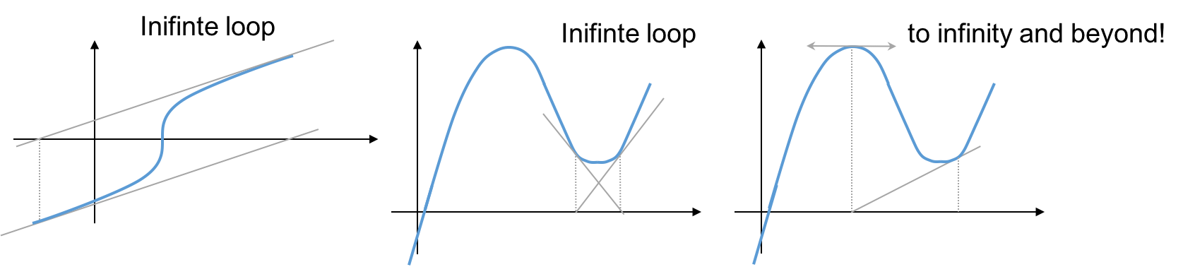
# ### Problem cases
#
#
#
# ### Problem cases
#  #
#
# ### Convergence
# $$x_{k+1}=x_k-\frac{f(x_k)}{f^{\prime}(x_k)}.$$
# * Subtract $x$ from both sides:
#
# $$\epsilon_{k+1} = \epsilon_k-\frac{f(x_k)}{f^{\prime}(x_k)}.$$
#
# * Taylor series: $$f(x) = f(x_k) + f^{\prime}(x_k)(x-x_k) + \frac{1}{2}f^{\prime\prime}(\xi)(x-x_k)^2.$$
# * Let $f(x)=0$ and $x_k-x = \epsilon_k$:
# $$f(x_k) = f^{\prime}(x_k)\epsilon_k - \frac{1}{2}f^{\prime\prime}(\xi)\epsilon_k^2,$$
# $$\frac{f(x_k)}{f^{\prime}(x_k)} = \epsilon_k - \frac{1}{2}\frac{f^{\prime\prime}(\xi)}{f^{\prime}(x_k)}\cdot\epsilon_k^2.$$
# * Insert this into the green equation above:
#
# $$\epsilon_{k+1} = \frac{1}{2}\frac{f^{\prime\prime}(\xi)}{f^{\prime}(x_k)}\cdot\epsilon_k^2.$$
#
#
# $$\epsilon_{k+1} = \frac{1}{2}\frac{f^{\prime\prime}(\xi)}{f^{\prime}(x_k)}\cdot\epsilon_k^2.$$
#
#
# * **Quadratic convergence**
# * Note, as $x_k\rightarrow x$, $\xi\rightarrow x$.
# * Takes a bit to get into the "quadratic" zone.
# * ...but once there, the number of significant digits roughly **doubles** at each iteration!
# * **Example**
# * Solve $f(x)= x^2-\pi^2 = 0$ for $x$.
# * One solution is at $x=\pi = 3.141592653589793$
# In[17]:
x = 1
print(f"x = {x:.15f}")
for k in range(6):
x = x - (x**2 - np.pi**2)/(2*x)
print(f"x = {x:.15f}")
# * k=0, x = 1.000000000000000
# * k=1, x = 5.434802200544679
# * k=2, x = **3**.625401431921964 $\rightarrow$ 1 digit
# * k=3, x = **3.1**73874724746142 $\rightarrow$ 2 digits
# * k=4, x = **3.141**756827069927 $\rightarrow$ 4 digits
# * k=5, x = **3.14159265**7879261 $\rightarrow$ 8 digits
# * k=6, x = **3.141592653589793** $\rightarrow$ 16 digits
# In[ ]:
#
#
# ### Convergence
# $$x_{k+1}=x_k-\frac{f(x_k)}{f^{\prime}(x_k)}.$$
# * Subtract $x$ from both sides:
#
# $$\epsilon_{k+1} = \epsilon_k-\frac{f(x_k)}{f^{\prime}(x_k)}.$$
#
# * Taylor series: $$f(x) = f(x_k) + f^{\prime}(x_k)(x-x_k) + \frac{1}{2}f^{\prime\prime}(\xi)(x-x_k)^2.$$
# * Let $f(x)=0$ and $x_k-x = \epsilon_k$:
# $$f(x_k) = f^{\prime}(x_k)\epsilon_k - \frac{1}{2}f^{\prime\prime}(\xi)\epsilon_k^2,$$
# $$\frac{f(x_k)}{f^{\prime}(x_k)} = \epsilon_k - \frac{1}{2}\frac{f^{\prime\prime}(\xi)}{f^{\prime}(x_k)}\cdot\epsilon_k^2.$$
# * Insert this into the green equation above:
#
# $$\epsilon_{k+1} = \frac{1}{2}\frac{f^{\prime\prime}(\xi)}{f^{\prime}(x_k)}\cdot\epsilon_k^2.$$
#
#
# $$\epsilon_{k+1} = \frac{1}{2}\frac{f^{\prime\prime}(\xi)}{f^{\prime}(x_k)}\cdot\epsilon_k^2.$$
#
#
# * **Quadratic convergence**
# * Note, as $x_k\rightarrow x$, $\xi\rightarrow x$.
# * Takes a bit to get into the "quadratic" zone.
# * ...but once there, the number of significant digits roughly **doubles** at each iteration!
# * **Example**
# * Solve $f(x)= x^2-\pi^2 = 0$ for $x$.
# * One solution is at $x=\pi = 3.141592653589793$
# In[17]:
x = 1
print(f"x = {x:.15f}")
for k in range(6):
x = x - (x**2 - np.pi**2)/(2*x)
print(f"x = {x:.15f}")
# * k=0, x = 1.000000000000000
# * k=1, x = 5.434802200544679
# * k=2, x = **3**.625401431921964 $\rightarrow$ 1 digit
# * k=3, x = **3.1**73874724746142 $\rightarrow$ 2 digits
# * k=4, x = **3.141**756827069927 $\rightarrow$ 4 digits
# * k=5, x = **3.14159265**7879261 $\rightarrow$ 8 digits
# * k=6, x = **3.141592653589793** $\rightarrow$ 16 digits
# In[ ]: