#!/usr/bin/env python
# coding: utf-8

# # Modeling Probabilities & Non-Linearities: Activation Functions
# 
# In this chapter, we will:
# 
# - Learn what is an activation function.
# - Learn about the standard hidden activation functions
#     - Sigmoid
#     - Tanh
# - Learn about the standard output activation functions
#     - Softmax
# 
# > [George Gordon Byron] "I Know that 2 and 2 make 4 –– & should be glad to prove it too if I could –– though I must say if by any sort of process I could convert 2 & 2 into 5 it would give me much greater pleasure"

# ## What is an Activation Function?

# An activation function is a function applied to the neurons in a layer during prediction. In that sense, an activation function is any function that can take one number and return another number. There are, however, an infinite number of functions in the universe, and not all of them are useful as activation functions. 
# 
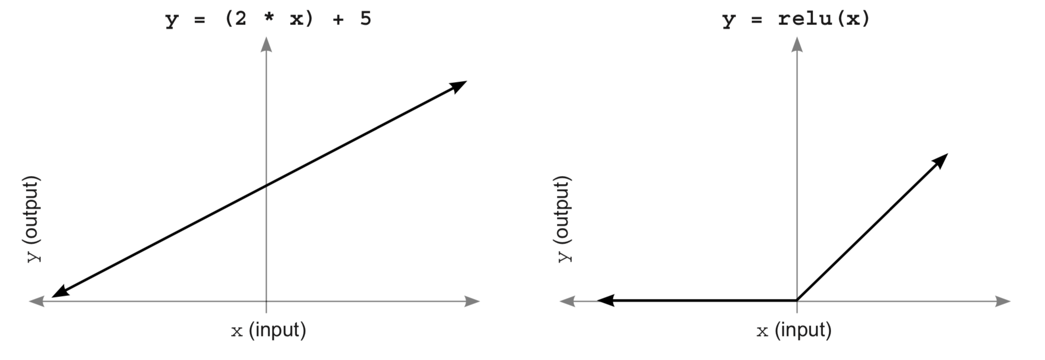
# We've already used an activation function called `ReLU`. The `ReLU` function had the effect of turning all negative numbers to zero.
# 
# There are many constraints on the nature of activation functions, we present them next.

# ### Constraint 1: The Function must be Continuous & Infinite in Domain
# 
# <div style="text-align:center"><img style="width:800px;" src="static/imgs/09/continuous-vs-non.png"></div>
# 
# 
# Meaning that the function must have an output number for any input.

# ### Constraint 2: Good Activation Functions are Monotonic (Increasing/Decreasing)
# 
# <div style="text-align:center"><img style="width:800px;" src="static/imgs/09/monotonic.png"></div>
# 
# An activation function must never change direction (always increasing/decreasing). This particular constrraint is not technically a requirement but if we consider a function that map different input values to the same output, then that function may have multiple perfect configurations. As a result, we can't know the correct direction to go.
# 
# For an advanced look into this subject, we should look more into convex versus non-convex optimization. 

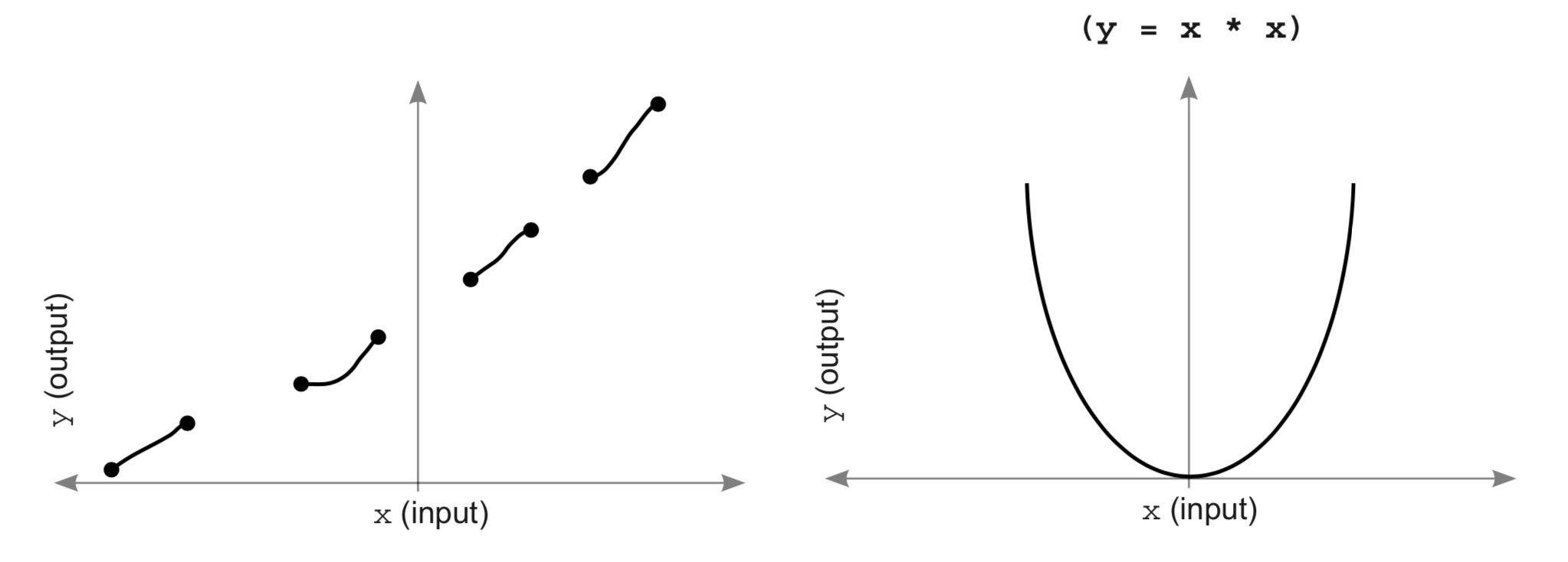
# ### Constraint 3: Good Activation Functions are Non-Linear
# 
# <div style="text-align:center"><img style="width:800px;" src="static/imgs/09/non-linearity.png"></div>
# 
# Linear functions scale values, they do not effect how correlated a neuron is to various inputs. They just make the collective corrrelation that is represented louder or softer.
# 
# What we want instead is **selective correlation**.

# ### Constraint 4: Good Activation Functions (& their derivatives) should be efficiently computable
# 
# We will be using the chosen activation functions a lot. For this reason, we want them (and their derivatives) to be efficiently computable. As an example, `ReLU` has become very popular mostly because it's efficient to compute. 

# ## Standard Hidden-Layer Activation Functions
# ### Which ones are most commonly used?

# ### Sigmoid is the bread & butter Activation
# 
# <div style="text-align:center"><img style="width:400px;" src="static/imgs/09/sigmoid.png"></div>
# 
# Sigmoid is great because it smoothly squinshes the infinite amount of input to an output between $0$ and $1$. This lets us interpret the output of any neuron as a **probability**. We typically use this non-linearity both in hidden and outputs layers.

# ### Tanh is better than sigmoid for hidden layers
# 
# <div style="text-align:center"><img style="width:400px;" src="static/imgs/09/tanh.png"></div>
# 
# `Tanh` is the same as sigmoid except it's between `-1` and `1`. This means it can also throw in some **negative** correlation. This aspect of negative correlation is powerful for hidden layers. On many problems, `tanh` will outperform sigmoid in the hidden layers.

# ## Standard output layer activation functions
# 
# For output layer activation functions, choosing the best one depends on what we're trying to predict. Broadly speaking, there are 3 major types of output layers:

# ### Configuration 1: Predicting Raw Data Values (Regression) — No activation function
# 
# One example might be predicting the average temperature in colorado given the average temperature in surrounding states.

# ### Configuration 2: Predicting Unrelated Yes/No Probabilities (Binary Classification) — Sigmoid
# 
# It's best to use the sigmoid function, Because it models individual probabilities separately for each output node.

# ### Configuration 3: Predicting which-one probabilities (Categorical Classification) — Softmax
# 
# This is by far the common use case in neural networks: predicting a single label out of many. In this case, it's better to have an activation function that models the idea that "The more likely it's one label, The less likely it's any of the other labels".

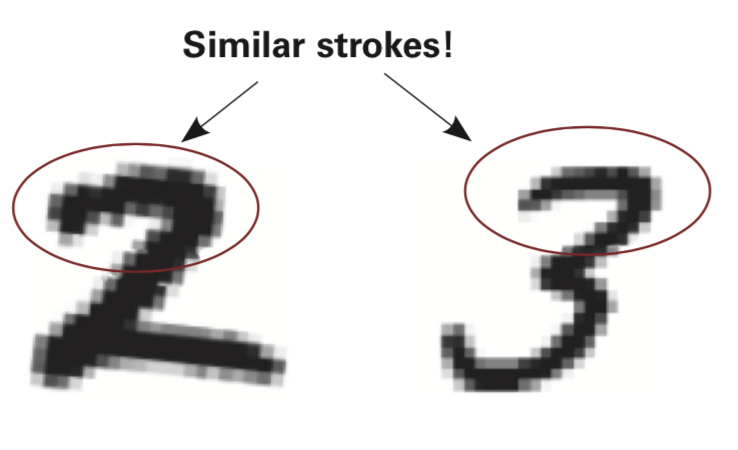
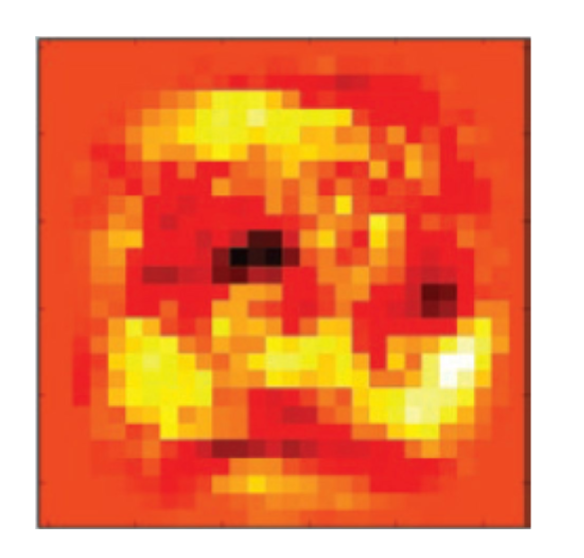
# ## The Core Issue: Inputs have similarity
# ### Different numbers share characteristics. It's good to let the network believe that
# 
# <div style="text-align:center">
#     <img style="width:33%;" src="static/imgs/09/similarity.png">
#     <img style="width:22%;" src="static/imgs/09/weights.png">
# </div>

# As we can see in the above figure, the average `2` shares quite a bit with the average `3`. As a general rule, similar inputs create similar outputs, when we take some numbers and multiply them by a matrix, if the starting numbers are pretty similar, the ending numbers will be pretty similar.
# 
# As a result, sigmoid will penelize the network for recognizing a `2` by anything other than features that are exclusively related to `2`s.
#     
# Most Images share lots of pixels in the middle of images. Because of that **the network will start trying to focus on the edges instead**. As we can see in the weight Image, the light areas are probably the best individual indicators of a `2`. 
# 
# What we are really striving for, though, is a network that "sees" the entire shape of a digit before outputing a prediction.

# ## Softmax Computation
# ### Softmax raises each input value exponentially and then divides by the layer's sum
# 
# $$\sigma(y)_{i} = \frac{e^{y_i}}{\sum_{j=1}^{K} e^{y_{j}}}$$
# 
# Softmax raises each input value exponentially and then divides by the layer's sum. The nice thing about softmax is that the higher the network predicts one value, the lower it predicts all the others. It encourages the network to pick out class with a very high probability.
# 
# To adjust how aggresively Softmax pushes the density to one class, use number slightly bigger or lower than $e$. Lower numbers will result in lower *attenuation* and higher numbers will result win bigger *attenuation*. For now, we stick to $e$.

# ## Activation Installation Instructions
# ### How do we add our favorite activation function to any layer?
# 
# We know the following:
# - The Slope of `ReLU` for positive numbers is exactly 1.
# - The Slope of `ReLU` for negative numbers is exactly 0.
# 
# As a reminder, the slope is a measure of how much the output of `ReLU` will change given a change in the input. The Input to a layer refers to the value before the nonlinearity. Modifying the input to `ReLU` (by a tiny amount) will have a 1:1 effect if it was predicting positively and a 0:1 effect if it was predicting negatively.
# 
# Thus, when we backpropagate, in order to generate `layer_1_delta`, multiply the backpropagated `delta` from `layer_2` (`layer_2_delta.dot(W_2.T)`) by the slope of `ReLU` at the point predicted in forward propagation. For some deltas the slope is $1$ (positive numbers) and for others it's $0$ (negative numbers).
# 
# The important thing to remember is that the slope is an indicator of how much a tiny change to the input effects the output. The update effect encourages the network to leave weights alone if adjusting them will have little to no effect.

# ## Multiplying Delta by the Slope
# 
# To compute `layer_delta`, we multiply the backpropagated delta by the layer's slope:
# 
# <div style="text-align:center">
#     <img style="width:33%;" src="static/imgs/09/layer_delta.png">
# </div>
# 
# `layer_1_delta[0]` represents how much higher or lower the first hidden node of layer 1 should be in order to reduce the error of the network. The end goal of delta on a neuron is to inform the weights whether they should move. If moving them would have no effect, they should be left alone.
# 
# <div style="text-align:center">
#     <img style="width:66%;" src="static/imgs/09/activations.png">
# </div>
# 
# This condition is obvious for ReLU, which is either on or off, but Sigmoid's sensitivity to change in the input slowly increases as the input approaches 0 from either direction. However, **very positive** and **very negative** inputs approach a slope of very near 0. Thus, as the input becomes very positive/negative, small changes to the incoming weights become less relevant to the neuron's error for the specific training example.

# ## Converting Output to Slope (Derivative)
# 
# For all of the previous activation functions, we can directly convert their output to their slope:
# 
# <div style="text-align:center">
#     <img style="width:75%;" src="static/imgs/09/Pariston.png">
# </div>
# 
# Most Great Activations have a means by which the output of the layer (at forward propagation) can be used to compute the derivative. This has become the standard practice for computing derivatives in neural networks, and it's quite handy.

# ## Upgrading the MNIST Network
# 
# Let's Upgrade the MNIST Network to reflect what you've learned. Theoretically, the `tanh` function should make for a better hidden-layer activation. The `softmax` function, on the other hand, should make for a better output layer activation function, but things aren't always as simple as they seem. For `Tanh` we had to reduce the standard diviation for the incoming weights (we adjust weigth values to be between `-.01` & `+.01`). We also tune the learning rate.

# In[1]:


import numpy as np
import sys


# In[2]:


from tensorflow.keras.datasets import mnist


# In[3]:


(X_train, y_train), (X_test, y_test) = mnist.load_data()
X_train.shape, y_train.shape, X_test.shape, y_test.shape


# In[4]:


images, labels = (X_train[:1000].reshape(1000, 28*28))/255, y_train[:1000]
images.shape, labels.shape


# In[5]:


one_hot_labels = np.zeros((labels.shape[0], 10))
one_hot_labels.shape


# In[6]:


for i, l in enumerate(labels):
    one_hot_labels[i][l] = 1
labels = one_hot_labels
labels.shape


# In[7]:


test_images = X_test.reshape(X_test.shape[0], 28*28)/255
test_images.shape


# In[8]:


one_hot_test_labels = np.zeros((y_test.shape[0], 10))
one_hot_test_labels.shape


# In[9]:


for i, l in enumerate(y_test):
    one_hot_test_labels[i][l] = 1
test_labels = one_hot_test_labels
test_labels.shape


# In[10]:


# activation functions.
def tanh(x):
    return np.tanh(x)

def tanh2deriv(output):
    return 1 - (output ** 2)

def softmax(x):
    temp = np.exp(x)
    return temp / np.sum(temp, axis=1, keepdims=True)


# In[11]:


alpha, iterations, hidden_size = (2, 300, 100)
pixels_per_image, num_labels = (784, 10)
batch_size = 100


# In[12]:


W_1 = (0.02 * np.random.random((pixels_per_image,hidden_size))) - 0.01
W_2 = (0.2 * np.random.random((hidden_size,num_labels))) - 0.1
W_1.shape, W_2.shape


# In[13]:


# Training Loop
for j in range(iterations):  # epoches
    correct_cnt = 0
    for i in range(int(len(images) / batch_size)):  # batches
        batch_start, batch_end = (i * batch_size), ((i+1) * batch_size)
        
        # Forward Propagation
        layer_0 = images[batch_start:batch_end]
        layer_1 = tanh(np.dot(layer_0, W_1))
        dropout_mask = np.random.randint(2,size=layer_1.shape)
        layer_1 *= dropout_mask * 2
        layer_2 = softmax(np.dot(layer_1, W_2))
        
        # benchmarking
        for k in range(batch_size):
            correct_cnt += int(np.argmax(layer_2[k:k+1]) == np.argmax(labels[batch_start+k:batch_start+k+1]))
        
        # backpropagation
        layer_2_delta = (labels[batch_start:batch_end] - layer_2) / (batch_size * layer_2.shape[0])
        layer_1_delta = layer_2_delta.dot(W_2.T)*tanh2deriv(layer_1)
        layer_1_delta *= dropout_mask
        
        # optimization
        W_2 += alpha * layer_1.T.dot(layer_2_delta)
        W_1 += alpha * layer_0.T.dot(layer_1_delta)
    
    test_correct_cnt = 0
    
    for i in range(len(test_images)):  # test images
        # predict
        layer_0 = test_images[i:i+1]
        layer_1 = tanh(np.dot(layer_0,W_1)) 
        layer_2 = np.dot(layer_1,W_2) 
        
        # benchmark
        test_correct_cnt += int(np.argmax(layer_2) == np.argmax(test_labels[i:i+1]))
    
    if(j % 10 == 0):
        print(f"I: {j} | Test-Acc: {round(test_correct_cnt / float(len(test_images)), 5)} | Train-Acc: {round(correct_cnt / float(len(images)), 5)}")


# ---

# ### ReLU + Dropout
# 
# In this section, we're going to make sure that we understand batch stochastic gradient descent + the new activation functions by implementing `Dropout` with `ReLU`:

# In[56]:


from tensorflow.keras import datasets 


# In[57]:


# Load Data.
(X_train, y_train), (X_test, y_test) = datasets.mnist.load_data()
X_train.shape, y_train.shape, X_test.shape, y_test.shape


# In[58]:


# light data pre-processing
x_train, y_train = (X_train[:1000].reshape((1000, 28*28))/255.), (y_train[:1000])


# In[59]:


# one hotting `y_train`
labels_train = np.zeros((y_train.shape[0], 10))
for i, v in enumerate(y_train):
    labels_train[i][v] = 1
labels_train[:3]


# In[60]:


# same to testing data.
x_test = X_test.reshape((-1, 28*28))/255.
labels_test = np.zeros((y_test.shape[0], 10))
for i, v in enumerate(y_test):
    labels_test[i][v] = 1
labels_test[:3]


# In[61]:


x_train.shape, labels_train.shape, x_test.shape, labels_test.shape


# In[62]:


# activation functions.
def ReLU(x):
    return (x > 0) * x

def grad_ReLU(x):
    return (x > 0).astype('int')

def tanh(x):
    return np.tanh(x)

def tanh2deriv(x):
    return 1 - (x ** 2)

def softmax(x):
    temp = np.exp(x)
    return temp / np.sum(temp, axis=1, keepdims=True)


# In[63]:


# configuration parameters
lr, epoches, hidden_size = 2, 100, 100
pixels_count, labels_count = 784, 10
batch_size = 100


# In[64]:


# Random Wights Initialization
W_0 = (0.02 * np.random.random((784,100))) - 0.01
W_1 = (0.02 * np.random.random((100,10))) - 0.01
W_0.shape, W_1.shape


# In[65]:


for epoch in range(epoches):
    
    # cuz each epoch passes through all training data, we calc error each epoch
    correct_count = []
    
    for batch_i in range(int(x_train.shape[0]/batch_size)):
        # get batch
        batch_start, batch_end = (batch_i * batch_size), ((batch_i+1) * batch_size)
        X = x_train[batch_start:batch_end]
        y = labels_train[batch_start:batch_end]
        
        # forward propagation
        layer_0 = X
        layer_1 = ReLU(np.matmul(layer_0, W_0))
        dropout_mask = np.random.randint(2, size=layer_1.shape)
        layer_1 *= dropout_mask * 2
        layer_2 = softmax(np.matmul(layer_1, W_1))
        
        # Evaluating, loop over the batch
        for k in range(batch_size):
            # we want to loop over the batch images.
            x_i, y_i, y_i_hat = X[k:k+1], y[k:k+1], layer_2[k:k+1]
            
            if np.argmax(y_i_hat.squeeze()) == np.argmax(y_i.squeeze()):
                correct_count.append(1)
            else:
                correct_count.append(0)
        
        # backpropagation
        layer_2_delta = (layer_2 - y) / (batch_size * layer_2.shape[1])
        layer_1_delta = layer_2_delta.dot(W_1.T) * grad_ReLU(layer_1)
        layer_1_delta *= dropout_mask
        
        # Optimization
        W_1 -= lr * (layer_1.T.dot(layer_2_delta))
        W_0 -= lr * (layer_0.T.dot(layer_1_delta))
        
    test_correct_count = list()
    
    # evaluate over test dataset.
    for i in range(x_test.shape[0]):
        # get data
        x_i, y_i = x_test[i:i+1], labels_test[i:i+1]
        
        # forward propagation
        layer_0 = x_i
        layer_1 = ReLU(layer_0.dot(W_0))
        layer_2 = softmax(layer_1.dot(W_1))
        
        if np.argmax(layer_2.squeeze()) == np.argmax(y_i.squeeze()):
            test_correct_count.append(1)
        else:
            test_correct_count.append(0)
        
    if(epoch % 10 == 0):
        print("\n"+ "Epoch:" + str(epoch) + \
              " Test-Acc:"+str(np.sum(np.array(test_correct_count))/np.array(test_correct_count).shape[0])+ \
              " Train-Acc:" + str(np.sum(np.array(correct_count))/np.array(correct_count).shape[0]))


# ---