#!/usr/bin/env python
# coding: utf-8
# # Free Body Diagram for Rigid Bodies
#
# > Renato Naville Watanabe
# > [Laboratory of Biomechanics and Motor Control](http://pesquisa.ufabc.edu.br/bmclab)
# > Federal University of ABC, Brazil
#
# ## Python setup
# In[1]:
import numpy as np
import matplotlib.pyplot as plt
# ## Equivalent systems
#
#
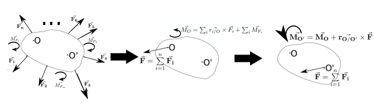
# A set of forces and moments is considered equivalent if its resultant force and sum of the moments computed relative to a given point are the same. Normally, we want to reduce all the forces and moments being applied to a body into a single force and a single moment.
#
# We have done this with particles for the resultant force. The resultant force is simply the sum of all the forces being applied to the body.
#
#
# \begin{equation}
# \vec{F} = \sum\limits_{i=1}^n \vec{F_i}
# \end{equation}
#
#
# where $\vec{F_i}$ is each force applied to the body.
#
# Similarly, the total moment applied to the body relative to a point O is:
#
#
# \begin{equation}
# \vec{M_O} = \sum\limits_{i}\vec{r_{i/O}} \times \vec{F_i}
# \end{equation}
#
#
# where $\vec{r_{i/O}}$ is the vector from the point O to the point where the force $\vec{\bf{F_i}}$ is being applied.
#
# But where the resultant force should be applied in the body? If the resultant force were applied to any point different from the point O, it would produce an additional moment to the body relative to point O. So, the resultant force must be applied to the point O.
#
# So, any set of forces can be reduced to a moment relative to a chosen point O and a resultant force applied to the point O.
#
# To compute the resultant force and moment relative to another point O', the new moment is:
#
#
# \begin{equation}
# \vec{M_{O'}} = \vec{M_O} + \vec{r_{O'/O}} \times \vec{F}
# \end{equation}
#
#
# And the resultant force is the same.
#
# It is worth to note that if the resultant force $\vec{F}$ is zero, than the moment is the same relative to any point.
#
#
# ## Steps to draw a free-body diagram
#
# The steps to draw the free-body diagram of a body is very similar to the case of particles.
#
# 1 - Draw separately each object considered in the problem. How you separate depends on what questions you want to answer.
# 2 - Identify the forces acting on each object. If you are analyzing more than one object, remember the third Newton law (action and reaction), and identify where the reaction of a force is being applied. Whenever a movement of translation of the body is constrained, a force at the direction of the constraint must exist.
# 3 - Identify the moments acting on each object. In the case you are analyzing more than one object, you must consider the action and reaction law (third Newton-Euler law). Whenever a movement of rotation of the body is constrained, a moment at the direction of the constraint must exist.
# 4 - Draw all the identified forces, representing them as vectors. The vectors should be represented with the origin in the object.
# 5 - Draw all the identified moments, representing them as vectors. In planar movements, the moments we be orthogonal to the considered plane. In these cases, normally the moment vectors are represented as curved arrows.
# 6 - If necessary, you should represent the reference frame (or references frames in case you use more than one reference frame) in the free-body diagram.
# 7 - After this, you can solve the problem using the First and Second Newton-Euler Laws (see, e.g, [Newton-Euler Laws](newton_euler_equations.ipynb)) to find the motion of the body.
#
#
# \begin{equation}
# \vec{F} = m\vec{a_{cm}} = m\frac{d^2\vec{r_{cm}}}{dt^2}
# \end{equation}
#
#
#
# \begin{equation}
# \vec{M_O} = I_{zz}^{cm}\vec{\alpha} + m \vec{r_{cm/O}} \times \vec{a_{cm}}=I_{zz}^{cm}\vec{\frac{d^2\theta}{dt^2}} + m \vec{r_{cm/O}} \times \frac{d^2\vec{r_{cm}}}{dt^2}
# \end{equation}
#
# ## Examples
#
# Below, we will see some examples of how to draw the free-body diagram and obtain the equation of motion.
# ### Horizontal fixed bar
#
# The first example is an example of statics. The bar has **no velocity** and **no acceleration**. We can find the **force** and **moment** the wall is applying to the bar.
#
#
# #### Free-body diagram
#
# The free-body diagram of the bar is depicted below. At the point where the bar is connected to the wall, there is a force $\vec{F_1}$ constraining the translation movement of the point O and a moment $\vec{M}$ constraining the rotation of the bar.
#
#
# #### Sum of the forces and moments
#
# The resultant force being applied to the bar is:
#
#
# \begin{equation}
# \vec{F} = -mg\hat{\bf{j}} + \vec{F_1}
# \end{equation}
#
#
# And the total moment in the z direction around the point O is:
#
#
# \begin{equation}
# \vec{M_O} = \vec{r_{C/O}}\times-mg\hat{\bf{j}} + \vec{M}
# \end{equation}
#
#
# The vector from the point O to the point C is given by $\vec{r_{C/O}} =\frac{l}{2}\hat{\bf{i}}$.
# #### Newton-Euler laws
# As the bar is fixed, all the accelerations are zero. So we can find the forces and the moment at the constraint.
#
#
# \begin{equation}
# \vec{F} = \vec{0}
# \end{equation}
#
#
#
# \begin{equation}
# -mg\hat{\bf{j}} + \vec{F_1} = \vec{0}
# \end{equation}
#
#
#
# \begin{equation}
# \vec{F_1} = mg\hat{\bf{j}}
# \end{equation}
#
#
#
# \begin{equation}
# \vec{M_O} = \vec{0}
# \end{equation}
#
#
#
# \begin{equation}
# \vec{r_{C/O}}\times-mg\hat{\bf{j}} + \vec{M} = \vec{0}
# \end{equation}
#
#
#
# \begin{equation}
# \frac{l}{2}\hat{\bf{i}}\times-mg\hat{\bf{j}} + \vec{M} = \vec{0}
# \end{equation}
#
#
#
# \begin{equation}
# -\frac{mgl}{2}\hat{\bf{k}} + \vec{M} = \vec{0}
# \end{equation}
#
#
#
# \begin{equation}
# \vec{M} = \frac{mgl}{2}\hat{\bf{k}}
# \end{equation}
#
# ### Rotating ball with drag force
#
#
# A **basketball** has a mass **$\bf{m = 0.63}$ kg** and radius equal $\bf{R = 12}$ **cm**. A basketball player shots the ball from the free-throw line (**4.6 m from the basket**) with a **speed of 9.5 m/s**, **angle of 51 degrees with the court**, **height of 2 m** and **angular velocity of 42 rad/s**. At the ball is acting a **drag force** $\bf{b_l = 0.5}$ **N.s/m** proportional to the modulus of the ball velocity in the opposite direction of the velocity and a **drag moment** $\bf{b_r = 0.001}$ **N.m.s**, proportional and in the opposite direction of the angular velocity of the ball. Consider the moment of inertia of the ball as $\bf{I_{zz}^{cm} = \frac{2mR^2}{3}}$.
# #### Free-body diagram
#
# Below is depicted the free-body diagram of the ball.
#
#
# #### Sum of forces and moments
#
# The resultant force being applied at the ball is:
#
#
# \begin{equation}
# \vec{F} = -mg\hat{\bf{j}} - b_l\vec{v} = -mg\hat{\bf{j}} - b_l\frac{d\vec{r}}{dt}
# \end{equation}
#
#
#
# \begin{equation}
# \vec{M_C} = - b_r\omega\hat{\bf{k}}=- b_r\frac{d\theta}{dt}\hat{\bf{k}}
# \end{equation}
#
# #### Newton-Euler laws
#
# So, by the second Newton-Euler law:
#
#
# \begin{equation}
# I_{zz}^{C}\frac{d^2\theta}{dt^2}=\vec{M_C}
# \end{equation}
#
#
#
# \begin{equation}
# I_{zz}^{C}\frac{d^2\theta}{dt^2} = - b_r\frac{d\theta}{dt}
# \end{equation}
#
#
# and by the first Newton-Euler law (for a revision on Newton-Euler laws, [see this notebook](newton_euler_equations.ipynb)):
#
#
# \begin{equation}
# m\frac{d^2\vec{r}}{dt^2}=\vec{F} \rightarrow \frac{d^2\vec{r}}{dt^2} = -g\hat{\bf{j}} - \frac{b_l}{m}\frac{d^2\vec{r}}{dt^2}
# \end{equation}
#
# #### Equations of motion
#
# So, we can split the differential equations above in three equations:
#
#
# \begin{equation}
# \frac{d^2\theta}{dt^2} = - \frac{b_r}{I_{zz}^{C}}\frac{d\theta}{dt}
# \end{equation}
#
#
#
# \begin{equation}
# \frac{d^2x}{dt^2} = - \frac{b_l}{m}\frac{dx}{dt}
# \end{equation}
#
#
#
# \begin{equation}
# \frac{d^2y}{dt^2} = -g - \frac{b_l}{m}\frac{dy}{dt}
# \end{equation}
#
# #### Numerical solution of the equations
#
# To solve these equations numerically, we can split each of these equations in first-order equations and the use a numerical method to integrate them. The first-order equations we be written in a matrix form, considering the moment of inertia of the ball as $I_{zz}^{C}=\frac{2mR^2}{3}$:
#
# \begin{equation}
# \left[\begin{array}{c}\frac{d\omega}{dt}\\\frac{dv_x}{dt}\\\frac{dv_y}{dt}\\\frac{d\theta}{dt}\\\frac{dx}{dt}\\\frac{dy}{dt} \end{array}\right] = \left[\begin{array}{c}- \frac{3b_r}{2mR^2}\omega\\- \frac{b_l}{m}v_x\\-g - \frac{b_l}{m}v_y\\\omega\\v_x\\v_y\end{array}\right]
# \end{equation}
#
#
# Below, the equations were solved numerically by using the Euler method (for a revision on numerical methods to solve ordinary differential equations, [see this notebook](OrdinaryDifferentialEquation.ipynb)).
# In[7]:
m = 0.63
R = 0.12
I = 2.0/3*m*R**2
bl = 0.5
br = 0.001
g = 9.81
x0 = 0
y0 = 2
v0 = 9.5
angle = 51*np.pi/180.0
vx0 = v0*np.cos(angle)
vy0 = v0*np.sin(angle)
dt = 0.001
t = np.arange(0, 2.1, dt)
x = x0
y = y0
vx = vx0
vy = vy0
omega = 42
theta = 0
r = np.array([x,y])
ballAngle = np.array([theta])
state = np.array([omega, vx, vy, theta, x, y])
while state[4]<=4.6:
dstatedt = np.array([-br/I*state[0],-bl/m*state[1], -g-bl/m*state[2],state[0], state[1], state[2] ])
state = state + dt * dstatedt
r = np.vstack((r, [state[4], state[5]]))
ballAngle = np.vstack((ballAngle, [state[3]]))
plt.figure(figsize=(10,8))
plt.plot(r[0:-1:50,0], r[0:-1:50,1], marker='o', color=np.array([1, 0.6,0]), markersize=17, linestyle='')
plt.plot(np.array([4, 4.45]), np.array([3.05, 3.05]))
for i in range(len(r[0:-1:50,0])):
plt.plot(r[i*50,0]+np.array([-0.05*(np.cos(ballAngle[i*50])-np.sin(ballAngle[i*50])),
0.05*(np.cos(ballAngle[i*50])-np.sin(ballAngle[i*50]))]),
r[i*50,1] + np.array([-0.05*(np.sin(ballAngle[i*50])+np.cos(ballAngle[i*50])),
0.05*(np.sin(ballAngle[i*50])+np.cos(ballAngle[i*50]))]),'k')
plt.ylim((0,4.5))
plt.show()
# Above is the trajectory of the ball until it reaches the basket (height of 3.05 m, marked with a blue line).
# ### Pendulum
#
# Now, we will analyze a **pendulum** of **lenght** $\bf{l}$. It consists of a bar with its **upper part linked to a hinge**.
#
#
# #### Free-body diagram
#
# Below is the free-body diagram of the bar. On the center of mass of the bar is acting the gravitational force. On the point O, where there is a hinge, a force $\vec{\bf{F_1}}$ restrains the point to translate. As the hinge does not constrains a rotational movement of the bar, there is no moment applied by the hinge.
#
#
# #### Sum of the forces and moments
#
# To find the equation of motion of the bar we can use the second Newton-Euler law. So, we must find the sum of the moments and the resultant force being applied to the bar. The sum of moments could be computed relative to any point, but if we choose the fixed point O, it is easier because we can ignore the force $\vec{\bf{F_1}}$.
#
# The moment around the fixed point is:
#
#
# \begin{equation}
# \vec{M_O} = \vec{r_{cm/O}} \times (-mg\hat{\bf{j}})
# \end{equation}
#
#
# The resultant force applied in the bar is:
#
#
# \begin{equation}
# \vec{F} = -mg\hat{\bf{j}} + \vec{F_1}
# \end{equation}
#
# #### Second Newton-Euler law
#
# The second Newton-Euler law is:
#
#
# \begin{equation}
# \vec{M_O} = \frac{d\vec{H_O}}{dt}
# \end{equation}
#
#
# The angular momentum derivative of the bar around point O is:
#
#
# \begin{equation}
# \frac{d\vec{H_O}}{dt} = I_{zz}^{cm} \frac{d^2\theta}{dt^2} \hat{\bf{k}} + m \vec{r_{cm/O}} \times \vec{a_{cm}}
# \end{equation}
#
# #### Kinematics
#
# The vector from point O to the center of mass is:
#
#
# \begin{equation}
# \vec{r_{cm/O}} = \frac{l}{2}\sin{\theta}\hat{\bf{i}}-\frac{l}{2}\cos{\theta}\hat{\bf{j}}
# \end{equation}
#
#
# The position of the center of mass is, considering the point O as the origin, equal to $\vec{\bf{r_{cm/O}}}$. So, the center of mass acceleration is obtained by deriving it twice.
#
#
# \begin{equation}
# \vec{v_{cm}} = \frac{\vec{r_{cm/O}}}{dt} = \frac{l}{2}(\cos{\theta}\hat{\bf{i}}+\sin{\theta}\hat{\bf{j}})\frac{d\theta}{dt}
# \end{equation}
#
#
#
# \begin{equation}
# \vec{a_{cm}} = \frac{l}{2}(-\sin{\theta}\hat{\bf{i}}+\cos{\theta}\hat{\bf{j}})\left(\frac{d\theta}{dt}\right)^2 + \frac{l}{2}(\cos{\theta}\hat{\bf{i}}+\sin{\theta}\hat{\bf{j}})\frac{d^2\theta}{dt^2}
# \end{equation}
#
# #### Sum of the moments
#
# So, the moment around the point O:
#
# \begin{equation}
# \vec{M_O} = \vec{r_{cm/O}} \times (-mg\hat{\bf{j}}) = \left(\frac{l}{2}\sin{\theta}\hat{\bf{i}}-\frac{l}{2}\cos{\theta}\hat{\bf{j}}\right) \times (-mg\hat{\bf{j}}) = \frac{-mgl}{2}\sin{\theta}\hat{\bf{k}}
# \end{equation}
# #### Derivative of the angular momentum
#
# And the derivative of the angular momentum is:
#
#
# \begin{equation}
# \begin{array}{l l}
# \frac{d\vec{H_O}}{dt} &=& I_{zz}^{cm} \frac{d^2\theta}{dt^2}\hat{\bf{k}} + m \frac{l}{2}(\sin{\theta}\hat{\bf{i}}-\cos{\theta}\hat{\bf{j}}) \times \left[ \frac{l}{2}(-\sin{\theta}\hat{\bf{i}}+\cos{\theta}\hat{\bf{j}})\left(\frac{d\theta}{dt}\right)^2 + \frac{l}{2}(\cos{\theta}\hat{\bf{i}}+\sin{\theta}\hat{\bf{j}})\frac{d^2\theta}{dt^2} \right] \\
# &=& I_{zz}^{cm} \frac{d^2\theta}{dt^2}\hat{\bf{k}} + m \frac{l^2}{4}\frac{d^2\theta}{dt^2} \hat{\bf{k}} \\
# &=& \left(I_{zz}^{cm} + \frac{ml^2}{4}\right)\frac{d^2\theta}{dt^2} \hat{\bf{k}}
# \end{array}
# \end{equation}
#
# #### The equation of motion
#
# Now, by using the Newton-Euler laws, we can obtain the differential equation that describes the bar angle along time:
#
#
# \begin{equation}
# \frac{d\vec{H_O}}{dt} = \vec{M_O} \rightarrow \frac{-mgl}{2}\sin{\theta} = \left(I_{zz}^{cm} + \frac{ml^2}{4}\right)\frac{d^2\theta}{dt^2} \rightarrow \frac{d^2\theta}{dt^2} = \frac{-2mgl}{\left(4I_{zz}^{cm} + ml^2\right)}\sin{\theta}
# \end{equation}
#
#
# The moment of inertia of the bar relative to its center of mass is $I_{zz}^{cm} = \frac{ml^2}{12}$ (for a revision on moment of inertia see [this notebook](CenterOfMassAndMomentOfInertia.ipynb)). So, the equation of motion of the pendulum is:
#
#
# \begin{equation}
# \frac{d^2\theta}{dt^2} = \frac{-3g}{2l}\sin{\theta}
# \end{equation}
#
# ### Inverted Pendulum
#
# At this example we analyze the inverted pendulum. It consists of a bar with **length** $\bf{l}$ with its lowest extremity linked to a hinge.
#
#
# #### Free-body diagram
#
# The free-body diagram of the bar is depicted below. At the point where the bar is linked to the hinge, a force $\vec{F_1}$ acts at the bar due to the restraint of the translation imposed to the point O by the hinge. Additionally, the gravitational force acts at the center of mass of the bar.
#
#
# #### Sum of the forces and moments
#
# Similarly to pendulum, in this case we can find the equation of motion of the bar by using the second Newton-Euler law. To do that we must find the sum of the moments and the resultant force being applied to the bar. The sum of moments could be computed relative to any point, but if we choose the fixed point O, it is easier because we can ignore the force $\vec{F_1}$.
#
# The moment around the fixed point is:
#
#
# \begin{equation}
# \vec{M_O} = \vec{r_{cm/O}} \times (-mg\hat{\bf{j}})
# \end{equation}
#
#
# The resultant force applied in the bar is:
#
#
# \begin{equation}
# \vec{F} = -mg\hat{\bf{j}} + \vec{F_1}
# \end{equation}
#
# #### Second Newton-Euler law
#
# The second Newton-Euler law is:
#
#
# \begin{equation}
# \vec{M_O} = \frac{d\vec{H_O}}{dt}
# \end{equation}
#
#
# The angular momentum derivative of the bar around point O is:
#
#
# \begin{equation}
# \frac{d\vec{H_O}}{dt} = I_{zz}^{cm} \frac{d^2\theta}{dt^2} \hat{\bf{k}} + m \vec{r_{cm/O}} \times \vec{a_{cm}}
# \end{equation}
#
# #### Kinematics
#
# The equations above are exactly the same of the pendulum example. The difference is in the kinematics of the bar. Now,the vector from point O to the center of mass is:
#
#
# \begin{equation}
# \vec{r_{cm/O}} = -\frac{l}{2}\sin{\theta}\hat{\bf{i}}+\frac{l}{2}\cos{\theta}\hat{\bf{j}}
# \end{equation}
#
#
# The position of the center of mass of the bar is equal to the vector $\vec{\bf{r_{cm/O}}}$, since the point O is with velocity zero relative to the global reference frame. So the center of mass acceleration can be obtained by deriving this vector twice:
#
#
# \begin{equation}
# \vec{v_{cm}} = \frac{\vec{r_{cm/O}}}{dt} = -\frac{l}{2}(\cos{\theta}\hat{\bf{i}}+\sin{\theta}\hat{\bf{j}})\frac{d\theta}{dt}
# \end{equation}
#
#
#
# \begin{equation}
# \vec{a_{cm}} = \frac{l}{2}(\sin{\theta}\hat{\bf{i}}-\cos{\theta}\hat{\bf{j}})\left(\frac{d\theta}{dt}\right)^2 - \frac{l}{2}(\cos{\theta}\hat{\bf{i}}+\sin{\theta}\hat{\bf{j}})\frac{d^2\theta}{dt^2}
# \end{equation}
#
# #### Sum of the moments
#
#
# So, the moment around the point O is:
#
#
# \begin{equation}
# \vec{M_O} = \vec{r_{cm/O}} \times (-mg\hat{\bf{j}}) = \left(-\frac{l}{2}\sin{\theta}\hat{\bf{i}}+\frac{l}{2}\cos{\theta}\hat{\bf{j}}\right) \times (-mg\hat{\bf{j}}) = \frac{mgl}{2}\sin{\theta} \hat{\bf{k}}
# \end{equation}
#
#
#
# #### Derivative of the angular momentum
#
#
# And the derivative of the angular momentum is:
#
#
# \begin{equation}
# \begin{array}{l l}
# \frac{d\vec{H_O}}{dt} &=& I_{zz}^{cm} \frac{d^2\theta}{dt^2} \hat{\bf{k}} + m \left(-\frac{l}{2}\sin{\theta}\hat{\bf{i}}+\frac{l}{2}\cos{\theta}\hat{\bf{j}}\right) \times \left[\frac{l}{2}(\sin{\theta}\hat{\bf{i}}-\cos{\theta}\hat{\bf{j}})\left(\frac{d\theta}{dt}\right)^2 - \frac{l}{2}(\cos{\theta}\hat{\bf{i}}+\sin{\theta}\hat{\bf{j}})\frac{d^2\theta}{dt^2}\right] \\
# &=& I_{zz}^{cm} \frac{d^2\theta}{dt^2} \hat{\bf{k}} + m \frac{l^2}{4}\frac{d^2\theta}{dt^2}\hat{\bf{k}} \\
# &=& \left(I_{zz}^{cm} + \frac{ml^2}{4}\right)\frac{d^2\theta}{dt^2}\hat{\bf{k}}
# \end{array}
# \end{equation}
#
# #### The equation of motion
#
#
# By using the Newton-Euler laws, we can find the equation of motion of the bar:
#
#
# \begin{equation}
# \frac{d\vec{H_O}}{dt} = \vec{M_O} \rightarrow \left(I_{zz}^{cm} + \frac{ml^2}{4}\right)\frac{d^2\theta}{dt^2} = \frac{mgl}{2}\sin{\theta} \rightarrow \frac{d^2\theta}{dt^2} = \frac{2mgl}{\left(4I_{zz}^{cm} + ml^2\right)}\sin(\theta)
# \end{equation}
#
#
# The moment of inertia of the bar is $I_{zz}^{cm} = \frac{ml^2}{12}$. So, the equation of motion of the bar is:
#
#
# \begin{equation}
# \frac{d^2\theta}{dt^2} = \frac{3g}{2l}\sin(\theta)
# \end{equation}
#
# ### Human quiet standing
#
# A very simple model of the human quiet standing (frequently used) is to use an inverted pendulum to model the human body. On [this notebook](http://nbviewer.jupyter.org/github/demotu/BMC/blob/master/notebooks/IP_Model.ipynb) there is a more comprehensive explanation of human standing. Consider the body as a rigid uniform bar with moment of inertia $I_{zz}^{cm} = \frac{m_Bh_G^2}{3}$.
#
#
#
# Adapted from [Elias, Watanabe and Kohn (2014)](https://journals.plos.org/ploscompbiol/article?id=10.1371/journal.pcbi.1003944).
# #### Free-body diagram
#
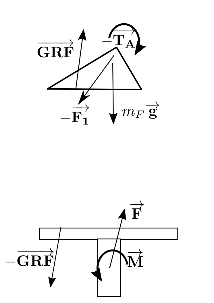
# Below is depicted the free-body diagram of the foot and the rest of the body. At the ankle joint there is a constraint to the translation of the ankle joint. So, a force $\vec{\bf{F_1}}$ is applied to the body at the ankle joint. By the third Newton law, a force $-\vec{\bf{F_1}}$ is applied to the foot at the ankle joint. At the center of mass of the body and of the foot, gravitational forces are applied. Additionally, a ground reaction force is applied to the foot at the center of pressure of the forces applied at the foot.
#
# Additionally, a moment $\vec{T_A}$ is applied at the body and its reaction is applied to the foot. This moment $\vec{T_A}$ comes from the muscles around the ankle joint. It is usual in Biomechanics to represent the net torque generated by all the muscles on a single joint as a single moment applied to the body.
#
#
# #### Sum of the moments
#
# The process to obtain the equation of motion of the body is very similar to the pendulums. The moment around the ankle being applied to the body is:
#
#
# \begin{equation}
# \vec{M_A} = \vec{T_A} + \vec{r_{cm/A}} \times (-m_Bg\hat{\bf{j}})
# \end{equation}
#
# #### Second Newton-Euler law
#
# And the derivative of the angular momentum is:
#
#
# \begin{equation}
# \frac{d\vec{H_A}}{dt} = I_{zz}^{cm}\frac{d^2\theta_A}{dt^2} + m\vec{r_{cm/A}} \times \vec{a_{cm}}
# \end{equation}
#
# #### Kinematics
#
# To find the kinematics of the bar, we could do the same procedure we have used in the pendulum and inverted pendulum examples, but this time we will use polar coordinates (for a revision on polar coordinates, see [Polar coordinates notebook](PolarCoordinates.ipynb)).
#
#
# \begin{equation}
# \vec{r_{cm/A}} = \vec{r_{cm}} = h_G\hat{\bf{e_r}}
# \end{equation}
#
#
#
# \begin{equation}
# \vec{v_{cm}} = h_G\frac{d\theta_A}{dt}\hat{\bf{e_\theta}}
# \end{equation}
#
#
#
# \begin{equation}
# \vec{a_{cm}} = -h_G\left(\frac{d\theta_A}{dt}\right)^2\hat{\bf{e_r}} + h_G\frac{d^2\theta_A}{dt^2}\hat{\bf{e_\theta}}
# \end{equation}
#
#
# where $\hat{\bf{e_r}} = -\sin(\theta_A)\hat{\bf{i}} + \cos(\theta_A)\hat{\bf{j}}$ and $\hat{\bf{e_\theta}} = -\cos(\theta_A)\hat{\bf{i}} - \sin(\theta_A)\hat{\bf{j}}$
# #### Sum of the moments
#
# Having the kinematics computed, we can go back to the moment and derivative of the angular momentum:
#
#
# \begin{equation}
# \vec{M_A} = \vec{T_A} + h_G\hat{\bf{e_r}} \times (-m_Bg\hat{\bf{j}}) = T_A\hat{\bf{k}} + h_Gm_Bg\sin(\theta_A)\hat{\bf{k}}
# \end{equation}
#
# ### Derivative of the angular momentum
#
#
# \begin{equation}
# \begin{array}{l l}
# \frac{d\vec{H_A}}{dt} &=& I_{zz}^{cm}\frac{d^2\theta_A}{dt^2} \hat{\bf{k}} + mh_G\hat{\bf{e_r}} \times \left(-h_G\left(\frac{d^2\theta_A}{dt^2}\right)^2\hat{\bf{e_r}} + h_G\frac{d^2\theta_A}{dt^2}\hat{\bf{e_\theta}}\right) \\
# &=& I_{zz}^{cm}\frac{d^2\theta_A}{dt^2}\hat{\bf{k}} + mh_G^2\frac{d^2\theta_A}{dt^2}\hat{\bf{k}} \\
# &=& \left(I_{zz}^{cm} + mh_G^2\right)\frac{d^2\theta_A}{dt^2}\hat{\bf{k}}
# \end{array}
# \end{equation}
#
# #### The equation of motion
#
# By using the Newton-Euler equations, we can now find the equation of motion of the body during quiet standing:
#
#
# \begin{equation}
# \vec{M_A}=\frac{d\vec{H_A}}{dt}
# \end{equation}
#
#
#
# \begin{equation}
# \left(I_{zz}^{cm} + mh_G^2\right)\frac{d^2\theta_A}{dt^2} = T_A + h_Gm_B g\sin(\theta_A)
# \end{equation}
#
#
#
# \begin{equation}
# \frac{d^2\theta_A}{dt^2} = \frac{h_Gm_B g}{I_{zz}^{cm} + mh_G^2}\sin(\theta_A)+ \frac{T_A}{I_{zz}^{cm} + m_Bh_G^2}
# \end{equation}
#
#
# If we consider the body as a rigid uniform bar, the moment of inertia is $I_{zz}^{cm} = \frac{m_Bh_G^2}{3}$. So, the equation of motion of the body is:
#
#
# \begin{equation}
# \frac{d^2\theta_A}{dt^2} = \frac{3 g}{4h_g}\sin(\theta_A)+ \frac{3 T_A}{4m_bh_G^2}
# \end{equation}
#
# ### Force platform (position of the center of pressure)
#
# From the same example above, now we will find the position of the center of pressure ($COP_x$) during the quiet standing. The $COP_x$ is the point where the ground reaction force is being applied. The point O is linked to the ground in a way that it constraints the translation and rotation movement of the platform and is located at known distance $y_0$ below the ground. Also, it is in the point O that sensors of force and moments are located.
#
#
#
# #### Free-body diagram
#
# The free-body diagram of the foot and the force platform is depicted below.
#
#
# In the platform , the distance $y_0$ is known. As the platform is in equilibrium its derivative of the angular momentum is zero. Now, we must find the sum of the moments. As we can choose any point, we will choose, the point where the force $\vec{\bf{F}}$ is being applied, and equal it to zero.
#
#
# \begin{equation}
# \vec{M} + \vec{r_{COP/O}} \times (-\vec{GRF}) = 0
# \end{equation}
#
#
# The vector $\vec{\bf{r_{COP/O}}}$ is:
#
#
# \begin{equation}
# \vec{r_{COP/O}} = COP_x \hat{\bf{i}} + y_0 \hat{\bf{j}}
# \end{equation}
#
#
# So, from the equation of the sum of the moments we can isolate the postion of the center of pressure:
#
#
# \begin{equation}
# M - COP_x GRF_y + y_0 GRF_x = 0 \rightarrow COP_x = \frac{M+y_0 GRF_x}{GRF_y}
# \end{equation}
#
#
# Using the expression above, we can track the position of the center of pressure during an experiment.
# ### Standing dummy (from Ruina and Pratap book)
#
# A standing dummy is modeled as having massless rigid circular feet of radius $R$ rigidly attached to their
# uniform rigid body of length $L$ and mass $m$. The feet do not slip on the floor.
#
#
#
#
# #### Free-body diagram
#
# Below is depicted the fee-body diagram. The point C is the point of contact with the ground. Note that this point changes its position along time, but instantly it has velocity zero.
#
#
# #### Kinematics
#
# Using the versors:
#
#
# \begin{equation}
# \hat{\bf{e_r}} = -\sin(\theta_A)\hat{\bf{i}} + \cos(\theta_A)\hat{\bf{j}}
# \end{equation}
#
#
#
# \begin{equation}
# \hat{\bf{e_\theta}} = -\cos(\theta_A)\hat{\bf{i}} - \sin(\theta_A)\hat{\bf{j}}
# \end{equation}
#
#
# The vector from the point C to the center of mass is:
#
#
# \begin{equation}
# \vec{r_{cm/C}} = R\hat{\bf{j}} + \left(\frac{L}{2} - R \right)\hat{\bf{e_r}}
# \end{equation}
#
#
# The position of the center of mass, relative to the origin is different from $\vec{r_{cm/C}}$. We can consider the origin of the system as the point of contact with the ground when the standing dummy is at the vertical position.
#
#
# \begin{equation}
# \vec{r_{cm}} = -R\theta\hat{\bf{i}} + R\hat{\bf{j}} + \left(\frac{L}{2} - R \right)\hat{\bf{e_r}}
# \end{equation}
#
#
#
# \begin{equation}
# \vec{v_{cm}} = -R\dot{\theta}\hat{\bf{i}} + \left(\frac{L}{2} - R \right)\dot{\theta}\hat{\bf{e_\theta}}
# \end{equation}
#
#
#
# \begin{equation}
# \vec{a_{cm}} = -R\ddot{\theta}\hat{\bf{i}} + \left(\frac{L}{2} - R \right)\ddot{\theta}\hat{\bf{e_\theta}} - \left(\frac{L}{2} - R \right)\dot{\theta}^2\hat{\bf{e_r}}
# \end{equation}
#
# #### Sum of the moments
#
#
# So, the moment around the point C is:
#
#
# \begin{equation}
# \vec{M_C} = \vec{r_{cm/C}} \times (-mg\hat{\bf{j}}) = \left[R\hat{\bf{j}} + \left(\frac{L}{2} - R \right)\hat{\bf{e_r}} \right] \times (-mg\hat{\bf{j}})
# \end{equation}
#
#
#
# \begin{equation}
# \vec{M_C} = mg\left(\frac{L}{2} - R \right)\sin{\theta}
# \end{equation}
#
# #### Derivative of the angular momentum
#
#
# \begin{equation}
# \begin{array}{l l}
# \dfrac{d\vec{H_C}}{dt} &=& I_{zz}^{cm}\ddot{\theta} \hat{\bf{k}} + m\vec{\bf{r_{cm/C}}} \times \vec{\bf{a_{cm}}} \\
# &=& \left[mR\hat{\bf{j}} + m\left(\frac{L}{2} - R \right)\hat{\bf{e_r}}\right] \times \left[-R\ddot{\theta}\hat{\bf{i}} + \left(\frac{L}{2} - R \right)\ddot{\theta}\hat{\bf{e_\theta}} - \left(\frac{L}{2} - R \right)\dot{\theta}^2\hat{\bf{e_r}}\right]
# \end{array}
# \end{equation}
#
#
#
# \begin{equation}
# \frac{d\vec{H_C}}{dt} = \left(I_{zz}^{cm}\ddot{\theta} + mR^2\ddot{\theta} + mR\left(\frac{L}{2} - mR \right)\ddot{\theta}\cos{\theta} - mR\left(\frac{L}{2} - mR \right)\dot{\theta}^2\sin{\theta} + mR\ddot{\theta}\left(\frac{L}{2} - R \right)\cos{\theta}+m\left(\frac{L}{2} - R \right)^2\ddot{\theta}\right)\hat{\bf{k}} = \left(I_{zz}^{cm}\ddot{\theta}+mR^2\ddot{\theta} + 2mR\left(\frac{L}{2} - R \right)\ddot{\theta}\cos{\theta} - mR\left(\frac{L}{2} - R \right)\dot{\theta}^2\sin{\theta} + m\left(\frac{L}{2} - R \right)^2\ddot{\theta}\right)\hat{\bf{k}} = \left(I_{zz}^{cm}\ddot{\theta} + mR^2\ddot{\theta} + m\left(RL - 2R^2 \right)\ddot{\theta}\cos{\theta} - m\left(\frac{RL}{2} - R^2 \right)\dot{\theta}^2\sin{\theta} + m\left(\frac{L^2}{4} - LR + R^2 \right)\ddot{\theta}\right)\hat{\bf{k}}
# \end{equation}
#
#
#
# \begin{equation}
# \frac{d\vec{H_C}}{dt} = \left(I_{zz}^{cm}+2mR^2 + mRL\cos{\theta} - 2mR^2\cos{\theta} + m\frac{L^2}{4}-mLR\right)\ddot{\theta} - m\left(\frac{RL}{2} - R^2 \right)\dot{\theta}^2\sin{\theta}
# \end{equation}
#
#
# Considering the moment of inertia of the bar as $I_{zz}^{cm} = \frac{mL^2}{12}$:
#
#
# \begin{equation}
# \frac{d\vec{H_C}}{dt} = \left(\frac{mL^2}{12}+2mR^2 + mRL\cos{\theta} - 2mR^2\cos{\theta} + \frac{mL^2}{4}-mLR\right)\ddot{\theta} - m\left(\frac{RL}{2} - R^2 \right)\dot{\theta}^2\sin{\theta}
# \end{equation}
#
#
#
# \begin{equation}
# \frac{d\vec{H_C}}{dt} = \left(\frac{mL^2}{3}+(2mR^2- mRL)(1-\cos{\theta})\right)\ddot{\theta} - m\left(\frac{RL}{2} - R^2 \right)\dot{\theta}^2\sin{\theta}
# \end{equation}
#
# #### The equation of motion
#
# By the second Newton-Euler law:
#
#
# \begin{equation}
# \left(2mL^2+(12mR^2- 6mRL)(1-\cos{\theta})\right)\ddot{\theta} - m\left(3RL - 6R^2 \right)\dot{\theta}^2\sin{\theta} = mg\left(3L - 6R \right)\sin{\theta}
# \end{equation}
#
#
#
# \begin{equation}
# \left(2L^2+(12R^2- 6RL)(1-\cos{\theta})\right)\ddot{\theta} = g\left(3L - 6R \right)\sin{\theta} + \left(3RL - 6R^2 \right)\dot{\theta}^2\sin{\theta}
# \end{equation}
#
#
#
# \begin{equation}
# \ddot{\theta} = \frac{3\left(L - 2R \right)\sin{\theta}\left(g + R\dot{\theta}^2\right)}{2L^2+(12R^2- 6RL)(1-\cos{\theta})}
# \end{equation}
#
#
# ### Double pendulum with actuators
#
# The figure below shows a double pendulum. This model can represent, for example, the arm and forearm of a subject.
#
#
# #### Free-body diagram
#
# The free-body diagrams of both bars are depicted below. There are constraint forces at all joints and moments from the muscles from both joints.
#
#
# #### Definition of versors
#
# The versors $\hat{\bf{e_{R_1}}}$, $\hat{\bf{e_{R_2}}}$, $\hat{\bf{e_{\theta_1}}}$ and $\hat{\bf{e_{\theta_2}}}$ are defined as:
#
#
# \begin{equation}
# \hat{\bf{e_{R_1}}} = \sin(\theta_1) \hat{\bf{i}} - \cos(\theta_1) \hat{\bf{j}}
# \end{equation}
#
#
#
# \begin{equation}
# \hat{\bf{e_{\theta_1}}} = \cos(\theta_1) \hat{\bf{i}} + \sin(\theta_1) \hat{\bf{j}}
# \end{equation}
#
#
#
# \begin{equation}
# \hat{\bf{e_{R_2}}} = \sin(\theta_2) \hat{\bf{i}} - \cos(\theta_2) \hat{\bf{j}}
# \end{equation}
#
#
#
# \begin{equation}
# \hat{\bf{e_{\theta_2}}} = \cos(\theta_2) \hat{\bf{i}} + \sin(\theta_2) \hat{\bf{j}}
# \end{equation}
#
# #### Kinematics
#
#
# \begin{equation}
# \vec{r_{C1/O1}} = \frac{l_1}{2} \hat{\bf{e_{R_1}}}
# \end{equation}
#
#
#
# \begin{equation}
# \vec{r_{O2/O1}} = l_1\hat{\bf{e_{R_1}}}
# \end{equation}
#
#
#
# \begin{equation}
# \vec{r_{C1}} = \vec{r_{C1/O1}} = \frac{l_1}{2} \hat{\bf{e_{R_1}}}
# \end{equation}
#
#
#
# \begin{equation}
# \vec{v_{C1}} = \frac{l_1}{2}\frac{d\theta_1}{dt}\hat{\bf{e_{\theta_1}}}
# \end{equation}
#
#
#
# \begin{equation}
# \vec{a_{C1}} = -\frac{l_1}{2}\left(\frac{d\theta_1}{dt}\right)^2 \hat{\bf{e_{R_1}}} + \frac{l_1}{2}\frac{d^2\theta_1}{dt^2} \hat{\bf{e_{\theta_1}}}
# \end{equation}
#
#
#
# \begin{equation}
# \vec{r_{C2/O2}} = \frac{l_2}{2}\hat{\bf{e_{R_2}}}
# \end{equation}
#
#
#
# \begin{equation}
# \vec{r_{C2}} = \vec{r_{O2/O1}} + \vec{r_{C2/O2}} = l_1\hat{\bf{e_{R_1}}} + \frac{l_2}{2}\hat{\bf{e_{R_2}}}
# \end{equation}
#
#
#
# \begin{equation}
# \vec{v_{C2}} = l_1\frac{d\theta_1}{dt}\hat{\bf{e_{\theta_1}}} + \frac{l_2}{2}\frac{d\theta_1}{dt}\hat{\bf{e_{\theta_2}}}
# \end{equation}
#
#
#
# \begin{equation}
# \vec{a_{C2}} = -l_1\left(\frac{d\theta_1}{dt}\right)^2 \hat{\bf{e_{R_1}}} + l_1\frac{d^2\theta_1}{dt^2} \hat{\bf{e_{\theta_1}}} -\frac{l_2}{2}\left(\frac{d\theta_2}{dt}\right)^2 \hat{\bf{e_{R_2}}} + \frac{l_2}{2}\frac{d^2\theta_2}{dt^2} \hat{\bf{e_{\theta_2}}}
# \end{equation}
#
# #### Sum of the moments of the lower bar around O2
#
# First, we can analyze the the sum of the moments and the derivative of the angular momentum at the lower bar relative to the point O2.
#
#
# \begin{equation}
# \vec{M_{O2}} = \vec{r_{C2/O2}} \times (-m_2g\hat{\bf{j}}) + \vec{M_{12}} = \frac{l_2}{2} \hat{\bf{e_{R_2}}} \times (-m_2g\hat{\bf{j}}) + \vec{M_{12}} = -\frac{m_2gl_2}{2}\sin(\theta_2)\hat{\bf{k}} + \vec{M_{12}}
# \end{equation}
#
# #### Derivative of angular momentum of the lower bar around O2
#
#
# \begin{equation}
# \frac{d\vec{H_{O2}}}{dt} = I_{zz}^{C2} \frac{d^2\theta_2}{dt^2} + m_2 \vec{r_{C2/O2}} \times \vec{a_{C2}} = I_{zz}^{C2} \frac{d^2\theta_2}{dt^2} + m_2 \frac{l_2}{2} \hat{\bf{e_{R_2}}} \times \left[-l_1\left(\frac{d\theta_1}{dt}\right)^2 \hat{\bf{e_{R_1}}} + l_1\frac{d^2\theta_1}{dt^2} \hat{\bf{e_{\theta_1}}} -\frac{l_2}{2}\left(\frac{d\theta_2}{dt}\right)^2 \hat{\bf{e_{R_2}}} + \frac{l_2}{2}\frac{d^2\theta_2}{dt^2} \hat{\bf{e_{\theta_2}}}\right]
# \end{equation}
#
#
# To complete the computation of the derivative of the angular momentum we must find the products
# $\hat{\bf{e_{R_2}}} \times \hat{\bf{e_{R_1}}} $, $\hat{\bf{e_{R_2}}} \times \hat{\bf{e_{\theta_1}}}$ and
# $\hat{\bf{e_{R_1}}} \times \hat{\bf{e_{\theta_2}}}$:
#
#
# \begin{equation}
# \hat{\bf{e_{R_2}}} \times \hat{\bf{e_{\theta_1}}} = \left[\begin{array}{c}\sin(\theta_2)\\-\cos(\theta_2)\end{array}\right] \times \left[\begin{array}{c}\cos(\theta_1)\\\sin(\theta_1)\end{array}\right] = \sin(\theta_1)\sin(\theta_2)+\cos(\theta_1)\cos(\theta_2) = \cos(\theta_1-\theta_2)
# \end{equation}
#
#
#
# \begin{equation}
# \hat{\bf{e_{R_2}}} \times \hat{\bf{e_{R_1}}} = \left[\begin{array}{c}\sin(\theta_2)\\-\cos(\theta_2)\end{array}\right] \times \left[\begin{array}{c}\sin(\theta_1)\\-\cos(\theta_1)\end{array}\right] = -\sin(\theta_2)\cos(\theta_1)+\cos(\theta_2)\sin(\theta_1) = \sin(\theta_1-\theta_2)
# \end{equation}
#
#
#
# \begin{equation}
# \hat{\bf{e_{R_1}}} \times \hat{\bf{e_{\theta_2}}} =\left[\begin{array}{c}\sin(\theta_1)\\-\cos(\theta_1)\end{array}\right] \times \left[\begin{array}{c}\cos(\theta_2)\\\sin(\theta_2)\end{array}\right] = \sin(\theta_2)\sin(\theta_1)+\cos(\theta_2)\cos(\theta_1) = \cos(\theta_1-\theta_2)
# \end{equation}
#
#
# So, the derivative of the angular momentum is:
#
#
# \begin{align}
# \begin{split}
# \frac{d\vec{H_{O2}}}{dt} &= I_{zz}^{C2} \frac{d^2\theta_2}{dt^2} - \frac{m_2l_1l_2}{2}\left(\frac{d\theta_1}{dt}\right)^2 \sin(\theta_1-\theta_2) + \frac{m_2l_1l_2}{2}\frac{d^2\theta_1}{dt^2} \cos(\theta_1-\theta_2) + \frac{m_2l_2^2}{4}\frac{d^2\theta_2}{dt^2} \\
# &= \frac{m_2l_1l_2}{2}\cos(\theta_1-\theta_2)\frac{d^2\theta_1}{dt^2} + \left(I_{zz}^{C2} + \frac{m_2l_2^2}{4} \right)\frac{d^2\theta_2}{dt^2}- \frac{m_2l_1l_2}{2}\left(\frac{d\theta_1}{dt}\right)^2 \sin(\theta_1-\theta_2)
# \end{split}
# \end{align}
#
# #### Sum of moments of the upper bar around O1
#
# Now we can analyze the sum of the moments and the derivative of the angular momentum at the upper bar. They will be computed relative to the point O1.
#
#
# \begin{equation}\begin{array}{l l}
# \vec{M_{O1}} &=& \vec{r_{C1/O1}} \times (-m_1g\hat{\bf{j}}) + \vec{r_{O2/O1}} \times (-\vec{F_{12}}) + \vec{M_{1}} - \vec{M_{12}} \\
# &=& \frac{l_1}{2} \hat{\bf{e_{R_1}}} \times (-m_1g\hat{\bf{j}}) + l_1\hat{\bf{e_{R_1}}} \times (-\vec{F_{12}}) + \vec{M_{1}} - \vec{M_{12}}
# \end{array}\end{equation}
#
#
#
# \begin{equation}
# \vec{M_{O1}}= \frac{-m_1gl_1}{2}\sin(\theta_1)\hat{\bf{k}} + l_1\hat{\bf{e_{R_1}}} \times (-\vec{F_{12}}) + \vec{M_{1}} - \vec{M_{12}}
# \end{equation}
#
#
# It remains to find the force
# $\vec{F_{12}}$ that is in the sum of moment of the upper bar. It can be found by finding the resultant force in the lower bar and use the First Newton-Euler law:
#
#
# \begin{equation}
# \vec{F_{12}} - m_2g \hat{\bf{j}} = m\vec{a_{C2}}
# \end{equation}
#
#
#
# \begin{equation}
# \vec{F_{12}} = m_2g \hat{\bf{j}} + m_2\left[-l_1\left(\frac{d\theta_1}{dt}\right)^2 \hat{\bf{e_{R_1}}} + l_1\frac{d^2\theta_1}{dt^2} \hat{\bf{e_{\theta_1}}} -\frac{l_2}{2}\left(\frac{d\theta_2}{dt}\right)^2 \hat{\bf{e_{R_2}}} + \frac{l_2}{2}\frac{d^2\theta_2}{dt^2} \hat{\bf{e_{\theta_2}}}\right]
# \end{equation}
#
#
# Now, we can go back to the moment $\vec{M_{O1}}$:
#
#
# \begin{align}
# \begin{split}
# \vec{M_{O1}} &= \frac{-m_1gl_1}{2}\sin(\theta_1)\hat{\bf{k}} + l_1\hat{\bf{e_{R_1}}} \times (-\vec{\bf{F_{12}}}) + \vec{M_{1}} - \vec{M_{12}} \\
# &= -\frac{m_1gl_1}{2}\sin(\theta_1)\hat{\bf{k}} - l_1\hat{\bf{e_{R_1}}} \times m_2\left[g \hat{\bf{j}}-l_1\left(\frac{d\theta_1}{dt}\right)^2 \hat{\bf{e_{R_1}}} + l_1\frac{d^2\theta_1}{dt^2} \hat{\bf{e_{\theta_1}}} -\frac{l_2}{2}\left(\frac{d\theta_2}{dt}\right)^2 \hat{\bf{e_{R_2}}} + \frac{l_2}{2}\frac{d^2\theta_2}{dt^2} \hat{\bf{e_{\theta_2}}}\right] + \vec{M_{1}} - \vec{M_{12}} \\
# &= -\frac{m_1gl_1}{2}\sin(\theta_1)\hat{\bf{k}} - m_2l_1g \sin(\theta_1)\hat{\bf{k}} - m_2l_1^2\frac{d^2\theta_1}{dt^2}\hat{\bf{k}} + \frac{m_2l_1l_2}{2}\left(\frac{d\theta_2}{dt}\right)^2 \sin(\theta_1-\theta_2)\hat{\bf{k}} - \frac{m_2l_1l_2}{2}\frac{d^2\theta_2}{dt^2} \cos(\theta_1-\theta_2)\hat{\bf{k}} + M_1\hat{\bf{k}} - M_{12}\hat{\bf{k}}
# \end{split}
# \end{align}
#
# #### Derivative of angular momentum of the upper bar around O1
#
#
# \begin{equation}
# \begin{array}{l l}
# \frac{d\vec{H_{O1}}}{dt} &=& I_{zz}^{C1} \frac{d^2\theta_1}{dt^2} + m_1 \vec{r_{C1/O1}} \times \vec{a_{C1}} \\
# &=& I_{zz}^{C1} \frac{d^2\theta_1}{dt^2} + m_1 \frac{l_1}{2} \hat{\bf{e_{R_1}}} \times \left[-\frac{l_1}{2}\left(\frac{d\theta_1}{dt}\right)^2 \hat{\bf{e_{R_1}}} + \frac{l_1}{2}\frac{d^2\theta_1}{dt^2} \hat{\bf{e_{\theta_1}}}\right]
# \end{array}
# \end{equation}
#
#
#
# \begin{equation}
# \frac{d\vec{H_{O1}}}{dt} =\left( I_{zz}^{C1} + m_1 \frac{l_1^2}{4}\right)\frac{d^2\theta_1}{dt^2}
# \end{equation}
#
# #### The equations of motion
#
# Finally, using the second Newton-Euler law for both bars, we can find the equation of motion of both angles:
#
#
# \begin{equation}
# \begin{array}{l l}
# \dfrac{d\vec{H_{O1}}}{dt} &=& \vec{M_{O1}} \rightarrow \left( I_{zz}^{C1} + m_1 \frac{l_1^2}{4}\right)\frac{d^2\theta_1}{dt^2} \\
# &=& -\frac{m_1gl_1}{2}\sin(\theta_1)- m_2l_1g \sin(\theta_1) - m_2l_1^2\frac{d^2\theta_1}{dt^2} + \frac{m_2l_1l_2}{2}\left(\frac{d\theta_2}{dt}\right)^2 \sin(\theta_1-\theta_2) - \frac{m_2l_1l_2}{2}\frac{d^2\theta_2}{dt^2} \cos{(\theta_1-\theta_2)} + M_1 - M_{12}
# \end{array}
# \end{equation}
#
#
#
# \begin{equation}
# \begin{array}{l l}
# \dfrac{d\vec{H_{O2}}}{dt} &=& \vec{M_{O2}} \rightarrow \frac{m_2l_1l_2}{2}\cos(\theta_1-\theta_2)\frac{d^2\theta_1}{dt^2} + \left(I_{zz}^{C2} + \frac{m_2l_2^2}{4} \right)\frac{d^2\theta_2}{dt^2}- \frac{m_2l_1l_2}{2}\left(\frac{d\theta_1}{dt}\right)^2 \sin(\theta_1-\theta_2) \\
# &=& -\frac{m_2gl_2}{2}\sin(\theta_2) + M_{12}
# \end{array}\end{equation}
#
#
# Considering the moment of inertia of the bars as $I_{zz}^{C1}=\frac{m_1l_1^2}{12}$ and $I_{zz}^{C2}=\frac{m_2l_2^2}{12}$ the differential equations above are:
#
#
# \begin{equation}
# \left(\dfrac{m_1l_1^2}{3} +m_2l_1^2\right)\frac{d^2\theta_1}{dt^2} + \frac{m_2l_1l_2}{2} \cos{(\theta_1-\theta_2)\frac{d^2\theta_2}{dt^2}} = -\frac{m_1gl_1}{2}\sin(\theta_1)- m_2l_1g \sin(\theta_1) + \frac{m_2l_1l_2}{2}\left(\frac{d\theta_2}{dt}\right)^2 \sin(\theta_1-\theta_2) + M_1 - M_{12}
# \end{equation}
#
#
#
# \begin{equation}
# \dfrac{m_2l_1l_2}{2}\cos(\theta_1-\theta_2)\frac{d^2\theta_1}{dt^2} + \frac{m_2l_2^2}{3}\frac{d^2\theta_2}{dt^2} = -\frac{m_2gl_2}{2}\sin(\theta_2) + \frac{m_2l_1l_2}{2}\left(\frac{d\theta_1}{dt}\right)^2 \sin(\theta_1-\theta_2)+ M_{12}
# \end{equation}
#
#
# We could isolate the angular accelerations but this would lead to very long equations.
# ## Further reading
#
# - Read the chapters 17 and 19 of the [Ruina and Rudra's book](http://ruina.tam.cornell.edu/Book/index.html).
# ## Video lectures on the internet
#
# - [Free Body Diagram for Rigid Body Equilibrium (I)](https://www.youtube.com/watch?v=go4vsgnb9jU);
# - [Free Body Diagram for Rigid Body Equilibrium (II)](https://www.youtube.com/watch?v=Qv2WoqJlIKQ);
# - [Free Body Diagram for Rigid Body Equilibrium (III)](https://www.youtube.com/watch?v=Knk068P-COg).
# ## Problems
#
# 1. Solve the problems 6, 7 and 8 from [this Notebook](FreeBodyDiagram.ipynb).
# 2. Solve the problems 17.2.9, 19.3.26, 19.3.29 from Ruina and Pratap book.
# 3. Study the content and solve the exercises of the text [Forces and Torques in Muscles and Joints](http://cnx.org/contents/d703853c-6382-4035-8d6a-dcbca00a15ca/Forces_and_Torques_in_Muscles_) (or [download here an off-line HTML copy of the content of that website](https://github.com/BMClab/BMC/blob/master/refs/forces-and-torques-in-muscles-and-joints-14.zip?raw=true)).
# ## References
#
# - Ruina A., Rudra P. (2019) [Introduction to Statics and Dynamics](http://ruina.tam.cornell.edu/Book/index.html). Oxford University Press.
#
# - Duarte M. (2017) [Free body diagram](FreeBodyDiagram.ipynb).
#
# - Elias, L A, Watanabe, R N, Kohn, A F.(2014) [Spinal Mechanisms May Provide a Combination of Intermittent and Continuous Control of Human Posture: Predictions from a Biologically Based Neuromusculoskeletal Model.](http://dx.doi.org/10.1371/journal.pcbi.1003944) PLOS Computational Biology (Online).
#
# - Winter D. A., (2009) Biomechanics and motor control of human movement. John Wiley and Sons.
#
# - Duarte M. (2017) [The inverted pendulum model of the human standing](http://nbviewer.jupyter.org/github/demotu/BMC/blob/master/notebooks/IP_Model.ipynb).