#!/usr/bin/env python
# coding: utf-8
# # Lagrangian mechanics
#
# > Marcos Duarte
# > [Laboratory of Biomechanics and Motor Control](http://pesquisa.ufabc.edu.br/bmclab)
# > Federal University of ABC, Brazil
#
# "The theoretical development of the laws of motion of bodies is a problem of such interest and importance, that it has engaged the attention of all the most eminent mathematicians, since the invention of dynamics as a mathematical science by Galileo, and especially since the wonderful extension which was given to that science by Newton. Among the successors of those illustrious men, Lagrange has perhaps done more than any other analyst, to give extent and harmony to such deductive researches, by showing that the most varied consequences respecting the motions of systems of bodies may be derived from one radical formula; the beauty of the method so suiting the dignity of the results, as to make of his great work a kind of scientific poem."Hamilton (1834)
#
# In[1]:
# import necessary libraries and configure environment
import numpy as np
import matplotlib.pyplot as plt
import seaborn as sns
sns.set_context('notebook', font_scale=1.2, rc={"lines.linewidth": 2})
# import Sympy functions
import sympy as sym
from sympy import Symbol, symbols, cos, sin, Matrix, simplify, Eq, latex, expand
from sympy.solvers.solveset import nonlinsolve
from sympy.physics.mechanics import dynamicsymbols, mlatex, init_vprinting
init_vprinting()
from IPython.display import display, Math
# ## Introduction
#
# We know that some problems in dynamics can be solved using the principle of conservation of mechanical energy, that the total mechanical energy in a system (the sum of potential and kinetic energies) is constant when only conservative forces are present in the system. Such approach is one kind of energy methods, see for example, pages 495-512 in Ruina and Pratap (2019).
#
# Lagrangian mechanics (after [Joseph-Louis Lagrange](https://en.wikipedia.org/wiki/Joseph-Louis_Lagrange)) can be seen as another kind of energy methods, but much more general, to the extent is an alternative to Newtonian mechanics.
#
# The Lagrangian mechanics is a formulation of classical mechanics where the equations of motion are obtained from the kinetic and potential energy of the system (scalar quantities) represented in generalized coordinates instead of using Newton's laws of motion to deduce the equations of motion from the forces on the system (vector quantities) represented in Cartesian coordinates.
# ## Generalized coordinates
#
# The direct application of Newton's laws to mechanical systems results in a set of equations of motion in terms of Cartesian coordinates of each of the particles that make up the system. In many cases, this is not the most convenient coordinate system to solve the problem or describe the movement of the system. For example, for a serial chain of rigid links, such as a member of the human body or from a robot manipulator, it may be simpler to describe the positions of each link by the angles between links.
#
# Coordinate systems such as angles of a chain of links are referred as [generalized coordinates](https://en.wikipedia.org/wiki/Generalized_coordinates). Generalized coordinates uniquely specify the positions of the particles in a system. Although there may be several generalized coordinates to describe a system, usually a judicious choice of generalized coordinates provides the minimum number of independent coordinates that define the configuration of a system (which is the number of degrees of freedom of the system), turning the problem simpler to solve. In this case, when the number of generalized coordinates equals the number of degrees of freedom, the system is referred as a holonomic system. In a non-holonomic system, the number of generalized coordinates necessary do describe the system depends on the path taken by the system.
#
# Being a little more technical, according to [Wikipedia](https://en.wikipedia.org/wiki/Configuration_space_(physics)):
# "In classical mechanics, the parameters that define the configuration of a system are called generalized coordinates, and the vector space defined by these coordinates is called the configuration space of the physical system. It is often the case that these parameters satisfy mathematical constraints, such that the set of actual configurations of the system is a manifold in the space of generalized coordinates. This manifold is called the configuration manifold of the system."
#
# In problems where it is desired to use generalized coordinates, one can write Newton's equations of motion in terms of Cartesian coordinates and then transform them into generalized coordinates. However, it would be desirable and convenient to have a general method that would directly establish the equations of motion in terms of a set of convenient generalized coordinates. In addition, general methods for writing, and perhaps solving, the equations of motion in terms of any coordinate system would also be desirable. The [Lagrangian mechanics](https://en.wikipedia.org/wiki/Lagrangian_mechanics) is such a method.
# ## Euler–Lagrange equations
#
#
# See [this notebook](http://nbviewer.jupyter.org/github/BMClab/bmc/blob/master/notebooks/lagrangian_mechanics_generalized.ipynb) for a deduction of the Lagrange's equation in generalized coordinates.
#
# Consider a system whose configuration (positions) can be described by a set of $N$ generalized coordinates $q_i\,(i=1,\dotsc,N)$.
#
# Let's define the Lagrange or Lagrangian function $\mathcal{L}$ as the difference between the total kinetic energy $T$ and the total potential energy $V$ of the system in terms of the generalized coordinates as:
#
#
# \begin{equation}
# \mathcal{L}(t,q,\dot{q}) = T(\dot{q}_1(t),\dotsc,\dot{q}_N(t)) - V(q_1(t),\dotsc,q_N(t))
# \label{}
# \end{equation}
#
#
# where the total potential energy is only due to conservative forces, that is, forces in which the total work done to move the system between two points is independent of the path taken.
#
# The Euler–Lagrange equations (or Lagrange's equations of the second kind) of the system are (omitting the functions' dependencies for sake of clarity):
#
#
# \begin{equation}
# \frac{\mathrm d }{\mathrm d t}\left( {\frac{\partial \mathcal{L}}{\partial \dot{q}_i }}
# \right)-\frac{\partial \mathcal{L}}{\partial q_i } = Q_{NCi} \quad i=1,\dotsc,N
# \label{}
# \end{equation}
#
#
# where $Q_{NCi}$ are the generalized forces due to non-conservative forces acting on the system, any forces that can't be expressed in terms of a potential.
#
# Once all derivatives of the Lagrangian function are calculated and substitute them in the equations above, the result is the equation of motion (EOM) for each generalized coordinate. There will be $N$ equations for a system with $N$ generalized coordinates.
# ### Steps to deduce the Euler-Lagrange equations
#
# 1. Model the problem. Define the number of degrees of freedom. Carefully select the corresponding generalized coordinates to describe the system;
# 2. Calculate the total kinetic and total potential energies of the system. Calculate the Lagrangian;
# 3. Calculate the generalized forces for each generalized coordinate;
# 4. For each generalized coordinate, calculate the three derivatives present on the left side of the Euler-Lagrange equation;
# 5. For each generalized coordinate, substitute the result of these three derivatives in the left side and the corresponding generalized forces in the right side of the Euler-Lagrange equation.
#
# The EOM's, one for each generalized coordinate, are the result of the last step.
# ### Example: Particle moving under the influence of a conservative force
#
# Let's deduce the EOM of a particle with mass $m$ moving in the three-dimensional space under the influence of a [conservative force](https://en.wikipedia.org/wiki/Conservative_force).
#
# The model is the particle moving in 3D space and there is no generalized force (non-conservative force); the particle has three degrees of freedom and we need three generalized coordinates, which can be $(x, y, z)$, where $y$ is vertical, in a Cartesian frame of reference.
# The Lagrangian $(\mathcal{L} = T - V)$ of the particle is:
#
#
# \begin{equation}
# \mathcal{L} = \frac{1}{2}m(\dot x^2(t) + \dot y^2(t) + \dot z^2(t)) - V(x(t),y(t),z(t))
# \label{}
# \end{equation}
#
#
# The equations of motion for the particle are found by applying the Euler–Lagrange equation for each coordinate.
# For the $x$ coordinate:
#
#
# \begin{equation}
# \frac{\mathrm d }{\mathrm d t}\left( {\frac{\partial \mathcal{L}}{\partial \dot{x}}}
# \right) - \frac{\partial \mathcal{L}}{\partial x } = 0
# \label{}
# \end{equation}
#
#
# And the derivatives are:
#
#
# \begin{equation}\begin{array}{l}
# m\ddot{x} + \dfrac{\partial V}{\partial x} = 0 \quad \rightarrow \\
# m\ddot{x} = -\dfrac{\partial V}{\partial x}
# \end{array}
# \label{}
# \end{equation}
#
#
# and same procedure for the $y$ and $z$ coordinates.
#
# The equation above is the Newton's second law of motion.
#
# For instance, if the conservative force is due to the gravitational field near Earth's surface $(V=[0, mgy, 0])$, the Euler–Lagrange equations (the EOM's) are:
#
#
# \begin{equation} \begin{array}{rcl}
# m\ddot{x} &=& -\dfrac{\partial (0)}{\partial x} &=& 0 \\
# m\ddot{y} &=& -\dfrac{\partial (mgy)}{\partial y} &=& -mg \\
# m\ddot{z} &=& -\dfrac{\partial (0)}{\partial z} &=& 0
# \end{array}
# \label{}
# \end{equation}
#
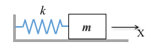
# ### Example: Ideal mass-spring system
#
#
#
# Consider a system with a mass $m$ attached to an ideal spring (massless, length $\ell_0$, and spring constant $k$) at the horizontal direction $x$. A force is momentarily applied to the mass and then the system is left unperturbed.
# Let's deduce the EOM of this system.
#
# The system can be modeled as a particle attached to a spring moving at the direction $x$, the only generalized coordinate needed (with origin of the Cartesian reference frame at the wall where the spring is attached), and there is no generalized force.
# The Lagrangian $(\mathcal{L} = T - V)$ of the system is:
#
#
# \begin{equation} \begin{array}{rcl}
# &\dfrac{\partial \mathcal{L}}{\partial x} &=& -k(x-\ell_0) \\
# &\dfrac{\partial \mathcal{L}}{\partial \dot{x}} &=& m\dot{x} \\
# &\dfrac{\mathrm d }{\mathrm d t}\left( {\dfrac{\partial \mathcal{L}}{\partial \dot{x}}} \right) &=& m\ddot{x}
# \end{array}
# \end{equation}
#
#
# Finally, the Euler–Lagrange equation (the EOM) is:
#
#
# \begin{equation}
# m\ddot{x} + k(x-\ell_0) = 0
# \label{}
# \end{equation}
#
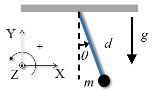
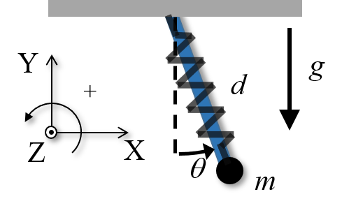
# ### Example: Simple pendulum under the influence of gravity
#
#
#
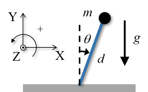
# Consider a pendulum with a massless rod of length $d$ and a mass $m$ at the extremity swinging in a plane forming the angle $\theta$ with the vertical.
# Let's deduce the EOM of this system.
#
# The model is a particle oscillating as a pendulum under a constant gravitational force $-mg$.
# Although the pendulum moves at the plane, it only has one degree of freedom, which can be described by the angle $\theta$, the generalized coordinate. Let's adopt the origin of the reference frame at the point of the pendulum suspension.
#
# The kinetic energy of the system is:
#
#
# \begin{equation}
# T = \frac{1}{2}mv^2 = \frac{1}{2}m(\dot{x}^2+\dot{y}^2)
# \end{equation}
#
#
# where $\dot{x}$ and $\dot{y}$ are:
#
#
# \begin{equation} \begin{array}{l}
# x = d\sin(\theta) \\
# y = -d\cos(\theta) \\
# \dot{x} = d\cos(\theta)\dot{\theta} \\
# \dot{y} = d\sin(\theta)\dot{\theta}
# \end{array} \end{equation}
#
#
# Consequently, the kinetic energy is:
#
#
# \begin{equation}
# T = \frac{1}{2}m\left((d\cos(\theta)\dot{\theta})^2 + (d\sin(\theta)\dot{\theta})^2\right) = \frac{1}{2}md^2\dot{\theta}^2
# \end{equation}
#
#
# And the potential energy of the system is:
#
#
# \begin{equation}
# V = -mgy = -mgd\cos\theta
# \end{equation}
#
#
# The Lagrangian function is:
#
#
# \begin{equation}
# \mathcal{L} = \frac{1}{2}md^2\dot\theta^2 + mgd\cos\theta
# \end{equation}
#
#
# And the derivatives are:
#
#
# \begin{equation} \begin{array}{rcl}
# &\dfrac{\partial \mathcal{L}}{\partial \theta} &=& -mgd\sin\theta \\
# &\dfrac{\partial \mathcal{L}}{\partial \dot{\theta}} &=& md^2\dot{\theta} \\
# &\dfrac{\mathrm d }{\mathrm d t}\left( {\dfrac{\partial \mathcal{L}}{\partial \dot{\theta}}} \right) &=& md^2\ddot{\theta}
# \end{array} \end{equation}
#
#
# Finally, the Euler–Lagrange equation (the EOM) is:
#
#
# \begin{equation}
# md^2\ddot\theta + mgd\sin\theta = 0
# \end{equation}
#
#
# Note that although the generalized coordinate of the system is $\theta$, we had to employ Cartesian coordinates at the beginning to derive expressions for the kinetic and potential energies. For kinetic energy, we could have used its equivalent definition for circular motion $(T=I\dot{\theta}^2/2=md^2\dot{\theta}^2/2)$, but for the potential energy there is no other way since the gravitational force acts in the vertical direction.
# In cases like this, a fundamental aspect is to express the Cartesian coordinates in terms of the generalized coordinates.
# #### Numerical solution of the equation of motion for the simple pendulum
#
# A classical approach to solve analytically the EOM for the simple pendulum is to consider the motion for small angles where $\sin\theta \approx \theta$ and the differential equation is linearized to $d\ddot\theta + g\theta = 0$. This equation has an analytical solution of the type $\theta(t) = A \sin(\omega t + \phi)$, where $\omega = \sqrt{g/d}$ and $A$ and $\phi$ are constants related to the initial position and velocity.
# For didactic purposes, let's solve numerically the differential equation for the pendulum using [Euler’s method](https://nbviewer.jupyter.org/github/demotu/BMC/blob/master/notebooks/OrdinaryDifferentialEquation.ipynb#Euler-method).
#
# Remember that we have to:
# 1. Transform the second-order ODE into two coupled first-order ODEs,
# 2. Approximate the derivative of each variable by its discrete first order difference
# 3. Write an equation to calculate the variable in a recursive way, updating its value with an equation based on the first order difference.
#
# We will also implement different variations of the Euler method: Forward (standard), Semi-implicit, and Semi-implicit variation (same results as Semi-implicit).
#
# Implementing these steps in Python:
# In[2]:
def euler_method(T=10, y0=[0, 0], h=.01, method=2):
"""
First-order numerical approximation for solving two coupled first-order ODEs.
A first-order differential equation is an initial value problem of the form:
y'(t) = f(t, y(t)) ; y(t0) = y0
Parameters:
T: total period (in s) of the numerical integration
y0: initial state [position, velocity]
h: step for the numerical integration
method: Euler method implementation, one of the following:
1: 'forward' (standard)
2: 'semi-implicit' (a.k.a., symplectic, Euler–Cromer)
3: 'semi-implicit variation' (same results as 'semi-implicit')
Two coupled first-order ODEs:
dydt = v
dvdt = a # calculate the expression for acceleration at each step
Two equations to update the values of the variables based on first-order difference:
y[i+1] = y[i] + h*v[i]
v[i+1] = v[i] + h*dvdt[i]
Returns arrays time, [position, velocity]
"""
N = int(np.ceil(T/h))
y = np.zeros((2, N))
y[:, 0] = y0
t = np.linspace(0, T, N, endpoint=False)
for i in range(N-1):
if method == 1: # forward (standard) Euler method
y[0, i+1] = y[0, i] + h*y[1, i]
y[1, i+1] = y[1, i] + h*dvdt(t[i], y[:, i])
elif method == 2: # semi-implicit Euler (Euler–Cromer) method
y[1, i+1] = y[1, i] + h*dvdt(t[i], y[:, i])
y[0, i+1] = y[0, i] + h*y[1, i+1]
elif method == 3: # variant of semi-implicit (equal results)
y[0, i+1] = y[0, i] + h*y[1, i]
y[1, i+1] = y[1, i] + h*dvdt(t[i], [y[0, i+1], y[1, i]])
else:
raise ValueError('Valid options for method are 1, 2, 3.')
return t, y
def dvdt(t, y):
"""
Returns dvdt at `t` given state `y`.
"""
d = 0.5 # length of the pendulum in m
g = 10 # acceleration of gravity in m/s2
return -g/d*np.sin(y[0])
def plot(t, y, labels):
"""
Plot data given in t, y, v with labels [title, ylabel@left, ylabel@right]
"""
fig, ax1 = plt.subplots(1, 1, figsize=(10, 4))
ax1.set_title(labels[0])
ax1.plot(t, y[0, :], 'b', label=' ')
ax1.set_xlabel('Time (s)')
ax1.set_ylabel(u'\u2014 ' + labels[1], color='b')
ax1.tick_params('y', colors='b')
ax2 = ax1.twinx()
ax2.plot(t, y[1, :], 'r-.', label=' ')
ax2.set_ylabel(u'\u2014 \u2027 ' + labels[2], color='r')
ax2.tick_params('y', colors='r')
plt.tight_layout()
plt.show()
# In[3]:
T, y0, h = 10, [45*np.pi/180, 0], .01
t, theta = euler_method(T, y0, h, method=2)
labels = ['Trajectory of simple pendulum under gravity',
'Angular position ($^o$)', 'Angular velocity ($^o/s$)']
plot(t, np.rad2deg(theta), labels)
# ### Python code to automate the calculation of the Euler–Lagrange equation
#
# The three derivatives in the Euler–Lagrange equations are first-order derivatives and behind the scenes we are using latex to write the equations. Both tasks are boring and error prone.
# Let's write a function using the Sympy library to automate the calculation of the derivative terms in the Euler–Lagrange equations and display them nicely.
# In[4]:
# helping function
def printeq(lhs, rhs=None):
"""Rich display of Sympy expression as lhs = rhs."""
if rhs is None:
display(Math(r'{}'.format(lhs)))
else:
display(Math(r'{} = '.format(lhs) + mlatex(simplify(rhs, ratio=1.7))))
def lagrange_terms(L, q, show=True):
"""Calculate terms of Euler-Lagrange equations given the Lagrangian and q's.
"""
if not isinstance(q, list):
q = [q]
Lterms = []
if show:
s = '' if len(q) == 1 else 's'
printeq(r"\text{Terms of the Euler-Lagrange equation%s:}"%(s))
for qi in q:
dLdqi = simplify(L.diff(qi))
Lterms.append(dLdqi)
dLdqdi = simplify(L.diff(qi.diff(t)))
Lterms.append(dLdqdi)
dtdLdqdi = simplify(dLdqdi.diff(t))
Lterms.append(dtdLdqdi)
if show:
printeq(r'\text{For generalized coordinate}\;%s:'%latex(qi.func))
printeq(r'\quad\dfrac{\partial\mathcal{L}}{\partial %s}'%latex(qi.func), dLdqi)
printeq(r'\quad\dfrac{\partial\mathcal{L}}{\partial\dot{%s}}'%latex(qi.func), dLdqdi)
printeq(r'\quad\dfrac{\mathrm d}{\mathrm{dt}}\left({\dfrac{'+
r'\partial\mathcal{L}}{\partial\dot{%s}}}\right)'%latex(qi.func), dtdLdqdi)
return Lterms
def lagrange_eq(Lterms, Qnc=None):
"""Display Euler-Lagrange equation given the Lterms."""
s = '' if len(Lterms) == 3 else 's'
if Qnc is None:
Qnc = int(len(Lterms)/3) * [0]
printeq(r"\text{Euler-Lagrange equation%s (EOM):}"%(s))
for i in range(int(len(Lterms)/3)):
#display(Eq(simplify(Lterms[3*i+2]-Lterms[3*i]), Qnc[i], evaluate=False))
printeq(r'\quad ' + mlatex(simplify(Lterms[3*i+2]-Lterms[3*i])), Qnc[i])
def lagrange_eq_solve(Lterms, q, Qnc=None):
"""Display Euler-Lagrange equation given the Lterms."""
if not isinstance(q, list):
q = [q]
if Qnc is None:
Qnc = int(len(Lterms)/3) * [0]
system = [simplify(Lterms[3*i+2]-Lterms[3*i]-Qnc[i]) for i in range(len(q))]
qdds = [qi.diff(t, 2) for qi in q]
sol = nonlinsolve(system, qdds)
s = '' if len(Lterms) == 3 else 's'
printeq(r"\text{Euler-Lagrange equation%s (EOM):}"%(s))
if len(sol.args):
for i in range(int(len(Lterms)/3)):
display(Eq(qdds[i], simplify(sol.args[0][i]), evaluate=False))
else:
display(sol)
return sol
# Let's recalculate the EOM of the simple pendulum using Sympy and the code for automation.
# In[5]:
# define variables
t = sym.Symbol('t')
m, d, g = sym.symbols('m, d, g', positive=True)
θ = dynamicsymbols('theta') # \theta
# Position and velocity of the simple pendulum under the influence of gravity:
# In[6]:
x, y = d*sin(𝜃), -d*cos(θ)
xd, yd = x.diff(t), y.diff(t)
printeq('x', x)
printeq('y', y)
printeq(r'\dot{x}', xd)
printeq(r'\dot{y}', yd)
# Kinetic and potential energies of the simple pendulum under the influence of gravity and the corresponding Lagrangian function:
# In[7]:
T = m*(xd**2 + yd**2)/2
V = m*g*y
printeq('T', T)
printeq('V', V)
L = T - V
printeq(r'\mathcal{L}', L)
# And the automated part for the derivatives:
# In[8]:
Lterms = lagrange_terms(L, θ)
# Finally, the EOM is:
# In[9]:
lagrange_eq(Lterms)
# And rearranging:
# In[10]:
sol = lagrange_eq_solve(Lterms, q=θ, Qnc=None)
# Same result as before.
# ### Example: Double pendulum under the influence of gravity
#
#
#
# Consider a double pendulum (one pendulum attached to another) with massless rods of length $d_1$ and $d_2$ and masses $m_1$ and $m_2$ at the extremities of each rod swinging in a plane forming the angles $\theta_1$ and $\theta_2$ with vertical.
# The system has two particles with two degrees of freedom; two adequate generalized coordinates to describe the system's configuration are the angles in relation to the vertical ($\theta_1, \theta_2$). Let's adopt the origin of the reference frame at the point of the upper pendulum suspension.
#
# Let's use Sympy to solve this problem.
# In[11]:
# define variables
t = Symbol('t')
d1, d2, m1, m2, g = symbols('d1, d2, m1, m2, g', positive=True)
θ1, θ2 = dynamicsymbols('theta1, theta2')
# The positions and velocities of masses $m_1$ and $m_2$ are:
# In[12]:
x1 = d1*sin(θ1)
y1 = -d1*cos(θ1)
x2 = d1*sin(θ1) + d2*sin(θ2)
y2 = -d1*cos(θ1) - d2*cos(θ2)
x1d, y1d = x1.diff(t), y1.diff(t)
x2d, y2d = x2.diff(t), y2.diff(t)
printeq(r'x_1', x1)
printeq(r'y_1', y1)
printeq(r'x_2', x2)
printeq(r'y_2', y2)
printeq(r'\dot{x}_1', x1d)
printeq(r'\dot{y}_1', y1d)
printeq(r'\dot{x}_2', x2d)
printeq(r'\dot{y}_2', y2d)
# The kinetic and potential energies of the system are:
# In[13]:
T = m1*(x1d**2 + y1d**2)/2 + m2*(x2d**2 + y2d**2)/2
V = m1*g*y1 + m2*g*y2
printeq(r'T', T)
printeq(r'V', V)
# The Lagrangian function is:
# In[14]:
L = T - V
printeq(r'\mathcal{L}', L)
# And the derivatives are:
# In[15]:
Lterms = lagrange_terms(L, [θ1, θ2])
# Finally, the EOM are:
# In[16]:
lagrange_eq(Lterms)
# The EOM's are a system with two coupled equations, $\theta_1$ and $\theta_2$ appear on both equations.
#
# The motion of a double pendulum is very interesting; most of times it presents a chaotic behavior.
# #### Numerical solution of the equation of motion for the double pendulum
#
# The analytical solution in infeasible to deduce. For the numerical solution, first we have to rearrange the equations to find separate expressions for $\theta_1$ and $\theta_2$ (solve the system of equations algebraically).
# Using Sympy, here are the two expressions:
# In[17]:
sol = lagrange_eq_solve(Lterms, q=[θ1, θ2], Qnc=None)
# In order to solve numerically the ODEs for the double pendulum we have to transform each equation above into two first ODEs. But we should avoid using Euler's method because of the non-negligible error in the numerical integration in this case; more accurate methods such as [Runge-Kutta](https://en.wikipedia.org/wiki/Runge%E2%80%93Kutta_methods) should be employed. See such solution in [https://www.myphysicslab.com/pendulum/double-pendulum-en.html](https://www.myphysicslab.com/pendulum/double-pendulum-en.html).
#
# We can use Sympy to transform the symbolic equations into Numpy functions that can be used for the numerical solution. Here is the code for that:
# In[18]:
θ1dd_fun = sym.lambdify((g, m1, d1, θ1, θ1.diff(t), m2, d2, θ2, θ2.diff(t)), sol.args[0][0], 'numpy')
θ2dd_fun = sym.lambdify((g, m1, d1, θ1, θ1.diff(t), m2, d2, θ2, θ2.diff(t)), sol.args[0][1], 'numpy')
# The reader is invited to write the code for the numerical simulation.
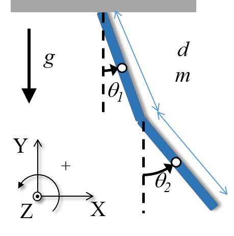
# ### Example: Double compound pendulum under the influence of gravity
#
#
#
# Consider the double compound pendulum (or physical pendulum) shown on the the right with length $d$ and mass $m$ of each rod swinging in a plane forming the angles $\theta_1$ and $\theta_2$ with vertical and $g=10 m/s^2$.
# The system has two degrees of freedom and we need two generalized coordinates ($\theta_1, \theta_2$) to describe the system's configuration.
#
# Let's use the Lagrangian mechanics to derive the equations of motion for each pendulum.
#
# To calculate the potential and kinetic energy of the system, we will need to calculate the position and velocity of each pendulum. Now each pendulum is a rod with distributed mass and we will have to calculate the moment of rotational inertia of the rod. In this case, the kinetic energy of each pendulum will be given as the kinetic energy due to rotation of the pendulum plus the kinetic energy due to the speed of the center of mass of the pendulum, such that the total kinetic energy of the system is:
#
# \begin{equation}\begin{array}{rcl}
# T = \overbrace{\underbrace{\,\frac{1}{2}I_{cm}\dot\theta_1^2\,}_{\text{rotation}} + \underbrace{\frac{1}{2}m(\dot x_{1,cm}^2 + \dot y_{1,cm}^2)}_{\text{translation}}}^{\text{pendulum 1}} + \overbrace{\underbrace{\,\frac{1}{2}I_{cm}\dot\theta_2^2\,}_{\text{rotation}} + \underbrace{\frac{1}{2}m(\dot x_{2,cm}^2 + \dot y_{2,cm}^2)}_{\text{translation}}}^{\text{pendulum 2}}
# \end{array}\end{equation}
#
# And the potential energy of the system is:
#
# \begin{equation}\begin{array}{rcl}
# V = mg\big(y_{1,cm} + y_{2,cm}\big)
# \end{array}\end{equation}
#
# Let's use Sympy once again.
#
# The position and velocity of the center of mass of the rods $1$ and $2$ are:
# In[19]:
d, m, g = symbols('d, m, g', positive=True)
θ1, θ2 = dynamicsymbols('theta1, theta2')
I = m*d*d/12 # rotational inertia of a rod
x1 = d*sin(θ1)/2
y1 = -d*cos(θ1)/2
x2 = d*sin(θ1) + d*sin(θ2)/2
y2 = -d*cos(θ1) - d*cos(θ2)/2
x1d, y1d = x1.diff(t), y1.diff(t)
x2d, y2d = x2.diff(t), y2.diff(t)
printeq(r'x_1', x1); printeq(r'y_1', y1)
printeq(r'x_2', x2); printeq(r'y_2', y2)
printeq(r'\dot{x}_1', x1d); printeq(r'\dot{y}_1', y1d)
printeq(r'\dot{x}_2', x2d); printeq(r'\dot{y}_2', y2d)
# The kinetic and potential energies of the system are:
# In[20]:
T = I/2*(θ1.diff(t))**2 + m/2*(x1d**2+y1d**2) + I/2*(θ2.diff(t))**2 + m/2*(x2d**2+y2d**2)
V = m*g*y1 + m*g*y2
printeq('T', T)
printeq('V', V)
# The Lagrangian function is:
# In[21]:
L = T - V
printeq(r'\mathcal{L}', L)
# And the derivatives are:
# In[22]:
Lterms = lagrange_terms(L, [θ1, θ2])
# Finally, the EOM are:
# In[23]:
lagrange_eq(Lterms)
# And rearranging:
# In[24]:
sol = lagrange_eq_solve(Lterms, q=[θ1, θ2], Qnc=None);
# ### Example: Double compound pendulum in joint space
#
# Let's recalculate the former example but employing generalized coordinates in the joint space: $\alpha_1=\theta_1$ and $\alpha_2=\theta_2-\theta_1$.
# In[25]:
d, m, g = symbols('d, m, g', positive=True)
α1, α2 = dynamicsymbols('alpha1, alpha2')
I = m*d*d/12 # rotational inertia of a rod
x1 = d*sin(α1)/2
y1 = -d*cos(α1)/2
x2 = d*sin(α1) + d*sin(α1+α2)/2
y2 = -d*cos(α1) - d*cos(α1+α2)/2
x1d, y1d = x1.diff(t), y1.diff(t)
x2d, y2d = x2.diff(t), y2.diff(t)
printeq(r'x_1', x1); printeq(r'y_1', y1)
printeq(r'x_2', x2); printeq(r'y_2', y2)
printeq(r'\dot{x}_1', x1d); printeq(r'\dot{y}_1', y1d)
printeq(r'\dot{x}_2', x2d); printeq(r'\dot{y}_2', y2d)
# In[26]:
T = I/2*(α1.diff(t))**2 + m/2*(x1d**2+y1d**2) + I/2*(α1.diff(t)+α2.diff(t))**2 + m/2*(x2d**2+y2d**2)
V = m*g*y1 + m*g*y2
L = T - V
printeq('T', T)
printeq('V', V)
printeq(r'\mathcal{L}', L)
# In[27]:
Lterms = lagrange_terms(L, [α1, α2])
# In[28]:
lagrange_eq(Lterms)
# In[29]:
sol = lagrange_eq_solve(Lterms, q=[α1, α2], Qnc=None)
# **Forces on the pendulum**
#
# We can see that besides the terms proportional to gravity $g$, there are three types of forces in the equations, two of these forces we already saw in the solution of the double pendulum employing generalized coordinates in the segment space: forces proportional to angular velocity squared $\dot{\theta}_i^2$ (now proportional to $\dot{\alpha}_i^2$) and forces proportional to the angular acceleration $\ddot{\theta}_i$ (now proportional to $\ddot{\alpha}_i$). These are the centripetal forces and tangential forces.
# A new type of force appeared explicitly in the equations when we employed generalized coordinates in the joint space: forces proportional to the product of the two angular velocities in joint space $\dot{\alpha}_1\dot{\alpha}_2$. These are the force of Coriolis.
# ### Example: Mass attached to a spring on a horizontal plane
#
#
#
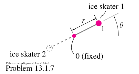
# Let's solve the exercise 13.1.7 of Ruina and Pratap (2019):
# "Two ice skaters whirl around one another. They are connected by a linear elastic cord whose center is stationary in space. We wish to consider the motion of one of the skaters by modeling her as a mass m held by a cord that exerts k Newtons for each meter it is extended from the central position.
# a) Draw a free-body diagram showing the forces that act on the mass is at an arbitrary position.
# b) Write the differential equations that describe the motion."
#
# Let's solve item b using Lagrangian mechanics.
#
# To calculate the potential and kinetic energy of the system, we will need to calculate the position and velocity of the mass. It's convenient to use as generalized coordinates, the radial position $r$ and the angle $\theta$.
#
# Using Sympy, declaring our parameters and coordinates:
# In[30]:
t = Symbol('t')
m, k = symbols('m, k', positive=True)
r, θ = dynamicsymbols('r, theta')
# The position and velocity of the skater are:
# In[31]:
x, y = r*cos(θ), r*sin(θ)
xd, yd = x.diff(t), y.diff(t)
printeq(r'x', x)
printeq(r'y', y)
printeq(r'\dot{x}', xd)
printeq(r'\dot{y}', yd)
# So, the kinetic and potential energies of the skater are:
# In[32]:
T = m*(xd**2 + yd**2)/2
V = (k*r**2)/2
display(Math('T=' + mlatex(T)))
display(Math('V=' + mlatex(V)))
printeq('T', T)
printeq('V', V)
# Where we considered the equilibrium length of the spring as zero.
#
# The Lagrangian function is:
# In[33]:
L = T - V
printeq(r'\mathcal{L}', L)
# And the derivatives are:
# In[34]:
Lterms = lagrange_terms(L, [r, θ])
# Finally, the EOM are:
# In[35]:
lagrange_eq(Lterms)
# In Ruina and Pratap's book they give as solution the equation: $2r\dot{r}\dot{\theta} + r^3\ddot{\theta}=0$, but using dimensional analysis we can check the book's solution is not correct.
# ## Generalized forces
#
# How non-conservative forces are treated in the Lagrangian Mechanics is different than in Newtonian mechanics.
# Newtonian mechanics consider the forces (and moment of forces) acting on each body (via FBD) and write down the equations of motion for each body/coordinate.
# In Lagrangian Mechanics, we consider the forces (and moment of forces) acting on each generalized coordinate. For such, the effects of the non-conservative forces have to be calculated in the direction of each generalized coordinate, these will be the generalized forces.
#
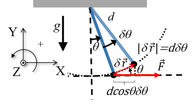
# A robust approach to determine the generalized forces on each generalized coordinate is to compute the work done by the forces to produce a small variation of the system on the direction of the generalized coordinate.
#
#
#
# For example, consider a pendulum with a massless rod of length $d$ and a mass $m$ at the extremity swinging in a plane forming the angle $\theta$ with the vertical.
# An external force acts on the tip of the pendulum at the horizontal direction.
# The pendulum cord is inextensible and the tip of the pendulum can only move along the arc of a circumference with radius $d$.
#
# The work done by this force to produce a small variation $\delta \theta$ is:
#
#
# \begin{equation}\begin{array}{l}
# \delta W_{NC} = \vec{F} \cdot \delta \vec{r} \\
# \delta W_{NC} = F d \cos(\theta) \delta \theta
# \end{array}
# \label{}
# \end{equation}
#
#
# We now reexpress the work as the product of the corresponding generalized force $Q_{NC}$ and the generalized coordinate:
#
#
# \begin{equation}
# \delta W_{NC} = Q_{NC} \delta \theta
# \label{}
# \end{equation}
#
#
# And comparing the last two equations, the generalized force (in fact, a moment of force) is:
#
#
# \begin{equation}
# Q_{NC} = F d \cos(\theta)
# \label{}
# \end{equation}
#
#
# Note that the work done by definition was expressed in Cartesian coordinates as the scalar product between vectors $\vec F$ and $\delta \vec{r}$ and after the scalar product was evaluated we end up with the work done expressed in terms of the generalized coordinate. This is somewhat similar to the calculation of kinetic and potential energy, these quantities are typically expressed first in terms of Cartesian coordinates, which in turn are expressed in terms of the generalized coordinates, so we end up with only generalized coordinates.
# Also note, we employ the term generalized force to refer to a non-conservative force or moment of force expressed in the generalized coordinate.
#
# If the force had components on both directions, we would calculate the work computing the scalar product between the variation in displacement and the force, as usual. For example, consider a force $\vec{F}=2\hat{i}+7\hat{j}$, the work done is:
#
#
# \begin{equation}\begin{array}{l}
# \delta W_{NC} = \vec{F} \cdot \delta \vec{r} \\
# \delta W_{NC} = [2\hat{i}+7\hat{j}] \cdot [d\cos(\theta) \delta \theta \hat{i} + d\sin(\theta) \delta \theta \hat{j}] \\
# \delta W_{NC} = d[2\cos(\theta) + 7\sin(\theta)] \delta \theta
# \end{array}
# \label{}
# \end{equation}
#
#
# Finally, the generalized force (a moment of force) is:
#
#
# \begin{equation}
# Q_{NC} = d[2\cos(\theta) + 7\sin(\theta)]
# \label{}
# \end{equation}
#
#
# For a system with $N$ generalized coordinates and $n$ non-conservative forces, to determine the generalized force at each generalized coordinate, we would compute the work as the sum of the works done by each force at each small variation:
#
#
# \begin{equation}
# \delta W_{NC} = \sum\limits_{j=1}^n F_{j} \cdot \delta x_j(\delta q_1, \dotsc, \delta q_N ) = \sum\limits_{i=1}^N Q_{i} \delta q_i
# \label{}
# \end{equation}
#
#
# For simpler problems, in which we can separately analyze each non-conservative force acting on each generalized coordinate, the work done by each force on a given generalized coordinate can be calculated by making all other coordinates immovable ('frozen') and then sum the generalized forces.
#
# The next examples will help to understand how to calculate the generalized force.
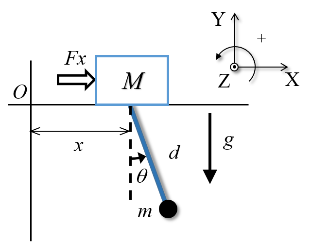
# ### Example: Simple pendulum on moving cart
#
#
#
# Consider a simple pendulum with massless rod of length $d$ and mass $m$ at the extremity of the rod forming an angle $\theta$ with the vertical direction under the action of gravity. The pendulum swings freely from a cart with mass $M$ that moves at the horizontal direction pushed by a force $F_x$.
#
# Let's use the Lagrangian mechanics to derive the EOM for the system.
#
# We will model the cart as a particle moving along the axis $x$, i.e., $y=0$. The system has two degrees of freedom and because of the constraints introduced by the constant length of the rod and the motion the cart can perform, good generalized coordinates to describe the configuration of the system are $x$ and $\theta$.
#
# **Determination of the generalized force**
# The force $F$ acts along the same direction of the generalized coordinate $x$, this means $F$ contributes entirely to the work done at the direction $x$. At this generalized coordinate, the generalized force due to $F$ is $F$.
# At the generalized coordinate $θ$, if we 'freeze' the generalized coordinate $x$ and let $F$ act on the system, there is no movement at the generalized coordinate $θ$, so no work is done. At this generalized coordinate, the generalized force due to $F$ is $0$.
#
# Let's now use Sympy to determine the EOM.
# The positions of the cart (c) and of the pendulum tip (p) are:
# In[36]:
t = Symbol('t')
M, m, d = symbols('M, m, d', positive=True)
x, y, θ, Fx = dynamicsymbols('x, y, theta, F_x')
# The positions of the cart (c) and of the pendulum tip (p) are:
# In[37]:
xc, yc = x, y*0
xcd, ycd = xc.diff(t), yc.diff(t)
xp, yp = x + d*sin(𝜃), -d*cos(θ)
xpd, ypd = xp.diff(t), yp.diff(t)
printeq(r'x_c', xc)
printeq(r'y_c', yc)
printeq(r'x_p', xp)
printeq(r'y_p', yp)
# The velocities of the cart and of the pendulum are:
# In[38]:
printeq(r'\dot{x}_c', xcd)
printeq(r'\dot{y}_c', ycd)
printeq(r'\dot{x}_p', xpd)
printeq(r'\dot{y}_p', ypd)
# The total kinetic and total potential energies and the Lagrangian of the system are:
# In[39]:
T = M*(xcd**2 + ycd**2)/2 + m*(xpd**2 + ypd**2)/2
V = M*g*yc + m*g*yp
printeq('T', T)
printeq('V', V)
L = T - V
printeq(r'\mathcal{L}', L)
# And the derivatives are:
# In[40]:
Lterms = lagrange_terms(L, [x, θ])
# Finally, the EOM are:
# In[41]:
lagrange_eq(Lterms, [Fx, 0])
# In[42]:
sol = lagrange_eq_solve(Lterms, q=[x, θ], Qnc=[Fx, 0])
# Note that although the force $F_x$ acts solely on the cart, the acceleration of the pendulum $\ddot{\theta}$ is also dependent on $F$, as expected.
#
# [Clik here for solutions to this problem using the Newtonian and Lagrangian approaches and how this system of two coupled second order differential equations can be rearranged for its numerical solution](http://www.emomi.com/download/neumann/pendulum_cart.html).
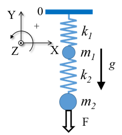
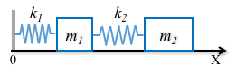
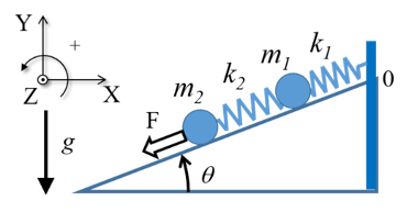
# ### Example: Two masses and two springs under the influence of gravity
#
#
#
# Consider a system composed by two masses $m_1,\, m_2$ and two ideal springs (massless, lengths $\ell_1,\, \ell_2$, and spring constants $k_1,\,k_2$) attached in series under gravity and a force $F$ acting directly on $m_2$.
#
# We can model this system as composed by two particles with two degrees of freedom and we need two generalized coordinates to describe the system's configuration; two obvious options are:
#
# - ${y_1, y_2}$, positions of masses $m_1,\, m_2$ w.r.t. ceiling (origin).
# - ${z_1, z_2}$, position of mass $m_1$ w.r.t. ceiling and position of mass $m_2$ w.r.t. mass $m_1$.
#
# The set ${y_1, y_2}$ is at an inertial reference frame, while the second set it's not.
# Let's find the EOM's using both sets of generalized coordinates and compare them.
#
# **Generalized forces**
# Using ${y_1, y_2}$, force $F$ acts on mass $m_2$ at the same direction of the generalized coordinate $y_2$. At this coordinate, the generalized force of $F$ is $F$. At the generalized coordinate $y_1$, if we 'freeze' the generalized coordinate $y_2$ and let $F$ act on the system, there is no movement at the generalized coordinate $y_1$ and no work is done. At this generalized coordinate, the generalized force due to $F$ is $0$.
#
# Using ${z_1, z_2}$, force $F$ acts on mass $m_2$ at the same direction of the generalized coordinate $z_2$. At this coordinate, the generalized force of $F$ is $F$. At the generalized coordinate $z_1$, if we 'freeze' the generalized coordinate $z_2$ and let $F$ act on the system, mass $m_1$ suffers the action of force $F$ at the generalized coordinate $y_1$. At this generalized coordinate, the generalized force due to $F$ is $F$.
#
# Sympy is our friend once again:
# In[43]:
t = Symbol('t')
m1, m2, ℓ01, ℓ02, g, k1, k2 = symbols('m1, m2, ell01, ell02, g, k1, k2', positive=True) # \ell
y1, y2, F = dynamicsymbols('y1, y2, F')
# The total kinetic and total potential energies of the system are:
# In[44]:
y1d, y2d = y1.diff(t), y2.diff(t)
T = (m1*y1d**2)/2 + (m2*y2d**2)/2
V = (k1*(y1-ℓ01)**2)/2 + (k2*((y2-y1)-ℓ02)**2)/2 - m1*g*y1 - m2*g*y2
printeq(r'T', T)
printeq(r'V', V)
# For sake of clarity, let's consider the resting lengths of the springs to be zero:
# In[45]:
V = V.subs([(ℓ01, 0), (ℓ02, 0)])
printeq(r'V', V)
# The Lagrangian function is:
# In[46]:
L = T - V
printeq(r'\mathcal{L}', L)
# And the derivatives are:
# In[47]:
Lterms = lagrange_terms(L, [y1, y2])
# Finally, the EOM are:
# In[48]:
lagrange_eq(Lterms, [0, F])
# In[49]:
lagrange_eq_solve(Lterms, [y1, y2], [0, F]);
# **Same problem, but with the other set of coordinates**
#
# Using ${z_1, z_2}$ as the position of mass $m_1$ w.r.t. the ceiling and the position of mass $m_2$ w.r.t. the mass $m_1$, the solution is:
# In[50]:
z1, z2 = dynamicsymbols('z1, z2')
z1d, z2d = z1.diff(t), z2.diff(t)
T = (m1*z1d**2)/2 + (m2*(z1d + z2d)**2)/2
V = (k1*(z1-ℓ01)**2)/2 + (k2*(z2-ℓ02)**2)/2 - m1*g*z1 - m2*g*(z1+z2)
printeq('T', T)
printeq('V', V)
# For sake of clarity, let's consider the resting lengths of the springs to be zero:
# In[51]:
V = V.subs([(ℓ01, 0), (ℓ02, 0)])
printeq(r'V', V)
# In[52]:
L = T - V
printeq(r'\mathcal{L}', L)
# In[53]:
Lterms = lagrange_terms(L, [z1, z2])
lagrange_eq(Lterms, [F, F])
# In[54]:
lagrange_eq_solve(Lterms, [z1, z2], [F, F]);
# The solutions using the two sets of coordinates seem different; the reader is invited to verify that in fact they are the same (remember that $y_1 = z_1,\, y_2 = z_1+z_2,\, \ddot{y}_2 = \ddot{z}_1+\ddot{z}_2$).
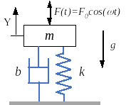
# ### Example: Mass-spring-damper system with gravity
#
#
#
# Consider a mass-spring-damper system under the action of the gravitational force and an external force acting on the mass.
# The massless spring has a stiffness coefficient $k$ and length at rest $\ell_0$.
# The massless damper has a damping coefficient $b$.
# The gravitational force acts downwards and it is negative (see figure).
# The system has one degree of freedom and we need only one generalized coordinate ($y$) to describe the system's configuration.
#
# There are two non-conservative forces acting at the direction of the generalized coordinate: the external force F and the force of the damper. By calculating the work done by each of these forces, the total generalized force is: $Q_{NC} = F_0 \cos(\omega t) - b\dot y$.
#
# Let's use the Lagrangian mechanics to derive the equations of motion for the system.
#
# The kinetic energy of the system is:
#
# \begin{equation}
# T = \frac{1}{2} m \dot y^2
# \end{equation}
#
# The potential energy of the system is:
#
# \begin{equation}
# V = \frac{1}{2} k (y-\ell_0)^2 + m g y
# \end{equation}
#
# The Lagrangian function is:
#
# \begin{equation}
# \mathcal{L} = \frac{1}{2} m \dot y^2 - \frac{1}{2} k (y-\ell_0)^2 - m g y
# \end{equation}
#
# The derivatives of the Lagrangian w.r.t. $y$ and $t$ are:
#
# \begin{equation}\begin{array}{rcl}
# \dfrac{\partial \mathcal{L}}{\partial y} &=& -k(y-\ell_0) - mg \\
# \dfrac{\partial \mathcal{L}}{\partial \dot{y}} &=& m \dot{y} \\
# \dfrac{\mathrm d }{\mathrm d t}\left( {\dfrac{\partial \mathcal{L}}{\partial \dot{y}}} \right) &=& m\ddot{y}
# \end{array}\end{equation}
#
# Substituting all these terms in the Euler-Lagrange equation, results in:
#
# \begin{equation}
# m\ddot{y} + b\dot{y} + k(y-\ell_0) + mg = F_0 \cos(\omega t)
# \end{equation}
# #### Numerical solution of the equation of motion for mass-spring-damper system
#
# Let's solve numerically the differential equation for the mass-spring-damper system with gravity using the function for the Euler's method we implemented before. We just have to write a new function for calculating the derivative of velocity:
# In[55]:
def dvdt(t, y):
"""
Returns dvdt at `t` given state `y`.
"""
m = 1 # mass, kg
k = 100 # spring coefficient, N/m
l0 = 1.0 # sprint resting length
b = 1.0 # damping coefficient, N/m/s
F0 = 2.0 # external force amplitude, N
f = 1 # frequency, Hz
g = 10 # acceleration of gravity, m/s2
F = F0*np.cos(2*np.pi*f*t) # external force, N
return (F - b*y[1] - k*(y[0]-l0) - m*g)/m
T, y0, h = 10, [1.1, 0], .01
t, y = euler_method(T, y0, h, method=2)
labels = ['Trajectory of mass-spring-damper system (Euler method)',
'Position (m)', 'Velocity (m/s)']
plot(t, y, labels)
# Here is the solution for this problem using the integration method explicit Runge-Kutta, a method with smaller errors in the integration and faster (for large amount of data) because the integration method in the Scipy function is implemented in Fortran:
# In[56]:
from scipy.integrate import solve_ivp
def dvdt2(t, y):
"""
Returns dvdt at `t` given state `y`.
"""
m = 1 # mass, kg
k = 100 # spring coefficient, N/m
l0 = 1.0 # sprint resting length
b = 1.0 # damping coefficient, N/m/s
F0 = 2.0 # external force amplitude, N
f = 1 # frequency, Hz
g = 10 # acceleration of gravity, m/s2
F = F0*np.cos(2*np.pi*f*t) # external force, N
return y[1], (F - b*y[1] - k*(y[0]-l0) - m*g)/m
T = 10.0 # s
freq = 100 # Hz
y02 = [1.1, 0.0] # [y0, v0]
t = np.linspace(0, T, int(T*freq), endpoint=False)
s = solve_ivp(fun=dvdt2, t_span=(t[0], t[-1]), y0=y02, method='RK45', t_eval=t)
labels = ['Trajectory of mass-spring-damper system (Runge-Kutta method)',
'Position (m)', 'Velocity (m/s)']
plot(s.t, s.y, labels)
# ## Forces of constraint
#
# The fact the Lagrangian formalism uses generalized coordinates means that in a system with constraints we typically have fewer coordinates (in turn, fewer equations of motion) and we don't need to worry about forces of constraint that we would have to consider in the Newtonian formalism.
# However, when we do want to determine a force of constraint, using Lagrangian formalism in fact will be disadvantageous! Let's see now one way of determining a force of constraint using Lagrangian formalism. The trick is to postpone the consideration that there is a constraint in the system; this will increase the number of generalized coordinates but will allow the determination of a force of constraint.
# Let's exemplify this approach determining the tension at the rod in the simple pendulum under the influence of gravity we saw earlier.
# ### Example: Force of constraint in a simple pendulum under the influence of gravity
#
#
#
# Consider a pendulum with a massless rod of length $d$ and a mass $m$ at the extremity swinging in a plane forming the angle $\theta$ with vertical and $g=10 m/s^2$.
#
# Although the pendulum moves at the plane, it only has one degree of freedom, which can be described by the angle $\theta$, the generalized coordinate. But because we want to determine the force of constraint tension at the rod, let's also consider for now the variable $r$ for the 'varying' length of the rod (instead of the constant $d$).
#
# In this case, the kinetic energy of the system will be:
#
#
# \begin{equation}
# T = \frac{1}{2}mr^2\dot\theta^2 + \frac{1}{2}m\dot r^2
# \end{equation}
#
#
# And for the potential energy we will also have to consider the constraining potential, $V_r(r(t))$:
#
#
# \begin{equation}
# V = -mgr\cos\theta + V_r(r(t))
# \end{equation}
#
#
# The Lagrangian function is:
#
#
# \begin{equation} \begin{array}{rcl}
# &\dfrac{\partial \mathcal{L}}{\partial r} &=& mr \dot\theta^2 + mg\cos\theta - \dot{V}_r(r) \\
# &\dfrac{\partial \mathcal{L}}{\partial \dot{r}} &=& m\dot r \\
# &\dfrac{\mathrm d }{\mathrm d t}\left( {\dfrac{\partial \mathcal{L}}{\partial \dot{r}}} \right) &=& m\ddot{r}
# \end{array} \end{equation}
#
#
# The Euler-Lagrange's equations (the equations of motion) are:
#
#
# \begin{equation} \begin{array}{rcl}
# &2mr\dot{r}\dot{\theta} + mr^2\ddot{\theta} + mgr\sin\theta &=& 0 \\
# &m\ddot{r} - mr \dot\theta^2 - mg\cos\theta + \dot{V}_r(r) &=& 0 \\
# \end{array} \end{equation}
#
#
# Now, we will apply the constraint condition, $r(t)=d$. This means that $\dot{r}=\ddot{r}=0$.
#
# With this constraint applied, the first Euler-Lagrange equation is the equation for the simple pendulum:
#
#
# \begin{equation}
# md^2\ddot{\theta} + mgd\sin\theta = 0
# \end{equation}
#
#
# The second equation yields:
#
#
# \begin{equation}
# -\dfrac{\mathrm d V_r}{\mathrm d r}\bigg{\rvert}_{r=d} = - md \dot\theta^2 - mg\cos\theta
# \end{equation}
#
#
# But the tension force, $F_T$, is by definition equal to the gradient of the constraining potential, so:
#
#
# \begin{equation}
# F_T = - md \dot\theta^2 - mg\cos\theta
# \end{equation}
#
#
# As expected, the tension at the rod is proportional to the centripetal and the gravitational forces.
# ## Lagrangian formalism applied to non-mechanical systems
#
# ### Example: Lagrangian formalism for RLC eletrical circuits
#
#
#
# It's possible to solve a RLC (Resistance-Inductance-Capacitance) electrical circuit using the Lagrangian formalism as an analogy with a mass-spring-damper system.
#
# In such analogy, the electrical charge is equivalent to position, current to velocity, inductance to mass, inverse of the capacitance to spring constant, resistance to damper constant (a dissipative element), and a generator would be analog to an external force actuating on the system. See the [Wikipedia](https://en.wikipedia.org/wiki/Mechanical%E2%80%93electrical_analogies) and [this paper](https://arxiv.org/pdf/1711.10245.pdf) for more details on this analogy.
#
# Let's see how to deduce the equivalent of equation of motion for a RLC series circuit (the Kirchhoff’s Voltage Law (KVL) equation).
#
#
#
# For a series RLC circuit, consider the following notation:
# $q$: charge
# $\dot{q}$: current admitted through the circuit
# $R$: effective resistance of the combined load, source, and components
# $C$: capacitance of the capacitor component
# $L$: inductance of the inductor component
# $u$: voltage source powering the circuit
# $P$: power dissipated by the resistance
#
# So, the equivalents of kinetic and potential energies are:
# $T = \frac{1}{2}L\dot{q}^2$
# $V = \frac{1}{2C}q^2$
# With a dissipative element:
# $P = \frac{1}{2}R\dot{q}^2$
# And the Lagrangian function is:
# $\mathcal{L} = \frac{1}{2}L\dot{q}^2 - \frac{1}{2C}q^2$
#
# Calculating the derivatives and substituting them in the Euler-Lagrange equation, we will have:
#
#
# \begin{equation}
# L \ddot{q} + R\dot{q} + \frac{q}{C} = u(t)
# \end{equation}
#
#
# Replacing $\dot{q}$ by $i$ and considering $v_c = q/C$ for a capacitor, we have the familar KVL equation:
#
#
# \begin{equation}
# L \frac{\mathrm d i}{\mathrm d t} + v_c + Ri = u(t)
# \end{equation}
#
# ## Considerations on the Lagrangian mechanics
#
# The Lagrangian mechanics does not constitute a new theory in classical mechanics; the results using Lagrangian or Newtonian mechanics must be the same for any mechanical system, only the method used to obtain the results is different.
#
# We are accustomed to think of mechanical systems in terms of vector quantities such as force, velocity, angular momentum, torque, etc., but in the Lagrangian formalism the equations of motion are obtained entirely in terms of the kinetic and potential energies (scalar operations) in the configuration space. Another important aspect of the force vs. energy analogy is that in situations where it is not possible to make explicit all the forces acting on the body, it is still possible to obtain expressions for the kinetic and potential energies.
#
# In fact, the concept of force does not enter into Lagrangian mechanics. This is an important property of the method. Since energy is a scalar quantity, the Lagrangian function for a system is invariant for coordinate transformations. Therefore, it is possible to move from a certain configuration space (in which the equations of motion can be somewhat complicated) to a space that can be chosen to allow maximum simplification of the problem.
# ## Further reading
#
# - [The Principle of Least Action](https://www.feynmanlectures.caltech.edu/II_19.html)
# - Vandiver JK (MIT OpenCourseWare) [An Introduction to Lagrangian Mechanics](https://ocw.mit.edu/courses/mechanical-engineering/2-003sc-engineering-dynamics-fall-2011/lagrange-equations/MIT2_003SCF11_Lagrange.pdf)
# ## Video lectures on the internet
#
# - iLectureOnline: [Lectures in Lagrangian Mechanics](http://www.ilectureonline.com/lectures/subject/PHYSICS/34/245)
# - MIT OpenCourseWare: [Introduction to Lagrange With Examples](https://youtu.be/zhk9xLjrmi4)
# ## Problems
#
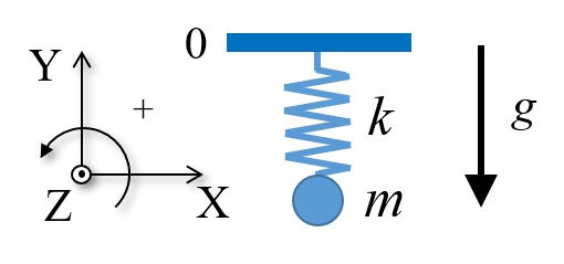
# 1. Derive the Euler-Lagrange equation (the equation of motion) for a mass-spring system where the spring is attached to the ceiling and the mass in hanging in the vertical (see solution for a system with two masses at https://youtu.be/dZjjzzWykio).
#
#
# 2. Derive the Euler-Lagrange equation for an inverted pendulum in the vertical.
#
#
# 3. Derive the Euler-Lagrange equation for the following system (see solution at https://youtu.be/8FSjEsUVNx8):
#
#
# 4. Derive the Euler-Lagrange equation for a spring pendulum, a simple pendulum where a mass $m$ is attached to a massless spring with spring constant $k$ and length at rest $d_0$ (see solution at https://youtu.be/iULa9A00JpA).
#
#
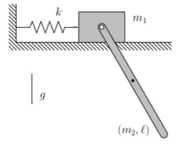
# 5. Derive the Euler-Lagrange equation for the system shown below (see solution for one mass spring system at https://youtu.be/eY0I8QK-ITE).
#
#
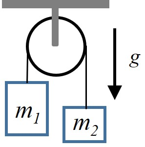
# 6. Derive the Euler-Lagrange equation for the following Atwood machine (consider that $m_1 > m_2$, i.e., the pulley will rotate counter-clockwise, and that moving down is in the positive direction) (see solution at https://youtu.be/lVg8I23Khz4):
#
#
# 7. Derive the Euler-Lagrange equation for the system below (see solution at https://youtu.be/gsi_0cVZ5-s):
#
#
# 8. Consider a person hanging by their hands from a bar and this person oscillates freely, behaving like a rigid pendulum under the action of gravity. The person's mass is $m$, the distance from their center of gravity to the bar is $r$, their rotational inertia is $I$, a line that passes through the bar and the person's body forms an angle $\theta$ with the vertical and the magnitude of the acceleration of gravity is $g$.
# a. Derive the equation of motion for the person's body using the Lagrangian formalism.
# b. If $m=100 kg $, $r=1 m$ and $g=10 m/s^2$ and the person takes $1 s$ to perform a complete oscillation, calculate an estimate for the rotational inertia.
# Tip: Use the approximation that for small angles $\sin\theta \approx \theta$ and solve the differential equation.
#
# 9. Consider a mass-spring system under the action of gravity where the spring is attached to the ceiling and the mass in hanging in the vertical. The spring's proportionality constant is $k = 2 N/m$ and its resting length is $\ell_0=1 m$. The mass attached to the spring is $2 kg$. Use $g = 10m/s^2$.
# a. Derive the differential equation that describes the movement of mass.
# b. Calculate the position of the mass over time considering that the spring is initially 2 m long and at rest.
# c. Write a pseudocode to calculate the position of the mass by numerical calculation using Euler's method to solve the differential equation.
#
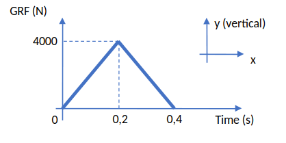
# 10. A widely used approach to study the interaction between the human body and the ground in locomotion is to model this interaction as a mass-spring-damper system with different quantities of these components. In an experiment to study this interaction during running, the vertical ground reaction force (GRF) was measured during the stance phase of a runner with a mass equal to $100 kg$ and the magnitude of GRF versus time is shown in the figure.
# a. Draw a free-body diagram for the runner's center of gravity.
# b. The maximum height of the runner in the aerial phase after the support phase shown in the graph above, knowing that the initial height and vertical speed (at $t=0 s$) of the runner (from his center of gravity) were $y_0 = 1 m$ and $v_0 = –2 m/s$.
# c. Draw the free-body diagram for a mechanical model of the corridor as a system consisting of a mass and spring and interaction with the ground.
# d. Derive the equation of motion for this model obtained in item c.
# e. Write a pseudocode to calculate the vertical trajectory from the differential equation obtained in item d by numerical calculation using Euler's method.
#
# 11. Write computer programs (in Python!) to solve numerically the equations of motion from the problems above.
# ## References
#
# - Hamilton WR (1834) [On a General Method in Dynamics](https://www.maths.tcd.ie/pub/HistMath/People/Hamilton/Dynamics/#GenMethod). Philosophical Transactions of the Royal Society, part II, 247-308.
# - Ruina A, Rudra P (2019) [Introduction to Statics and Dynamics](http://ruina.tam.cornell.edu/Book/index.html). Oxford University Press.