# Tensorflow Probability is part of the colab default runtime,
so you don't need to install Tensorflow or Tensorflow Probability if you're running this in the colab.
#
# If you're running this notebook in Jupyter on your own machine (and you have already installed Tensorflow), you can use the following
#
#
# - For the most recent nightly installation:
pip3 install -q tfp-nightly
# - For the most recent stable TFP release:
pip3 install -q --upgrade tensorflow-probability
# - For the most recent stable GPU-connected version of TFP:
pip3 install -q --upgrade tensorflow-probability-gpu
# - For the most recent nightly GPU-connected version of TFP:
pip3 install -q tfp-nightly-gpu
#
# Again, if you are running this in a Colab, Tensorflow and TFP are already installed
#
 Run in Google Colab
#
Run in Google Colab
#  View source on GitHub
#
View source on GitHub
#  #
#
# How would you determine which submissions are the best? There are a number of ways to achieve this:
#
# 1. *Popularity*: A submission is considered good if it has many upvotes. A problem with this model is that a submission with hundreds of upvotes, but thousands of downvotes. While being very *popular*, the submission is likely more controversial than best.
# 2. *Difference*: Using the *difference* of upvotes and downvotes. This solves the above problem, but fails when we consider the temporal nature of submission. Depending on when a submission is posted, the website may be experiencing high or low traffic. The difference method will bias the *Top* submissions to be the those made during high traffic periods, which have accumulated more upvotes than submissions that were not so graced, but are not necessarily the best.
# 3. *Time adjusted*: Consider using Difference divided by the age of the submission. This creates a *rate*, something like *difference per second*, or *per minute*. An immediate counter-example is, if we use per second, a 1 second old submission with 1 upvote would be better than a 100 second old submission with 99 upvotes. One can avoid this by only considering at least t second old submission. But what is a good t value? Does this mean no submission younger than t is good? We end up comparing unstable quantities with stable quantities (young vs. old submissions).
# 3. *Ratio*: Rank submissions by the ratio of upvotes to total number of votes (upvotes plus downvotes). This solves the temporal issue, such that new submissions who score well can be considered Top just as likely as older submissions, provided they have many upvotes to total votes. The problem here is that a submission with a single upvote (ratio = 1.0) will beat a submission with 999 upvotes and 1 downvote (ratio = 0.999), but clearly the latter submission is *more likely* to be better.
#
# I used the phrase *more likely* for good reason. It is possible that the former submission, with a single upvote, is in fact a better submission than the later with 999 upvotes. The hesitation to agree with this is because we have not seen the other 999 potential votes the former submission might get. Perhaps it will achieve an additional 999 upvotes and 0 downvotes and be considered better than the latter, though not likely.
#
# What we really want is an estimate of the *true upvote ratio*. Note that the true upvote ratio is not the same as the observed upvote ratio: the true upvote ratio is hidden, and we only observe upvotes vs. downvotes (one can think of the true upvote ratio as "what is the underlying probability someone gives this submission a upvote, versus a downvote"). So the 999 upvote/1 downvote submission probably has a true upvote ratio close to 1, which we can assert with confidence thanks to the Law of Large Numbers, but on the other hand we are much less certain about the true upvote ratio of the submission with only a single upvote. Sounds like a Bayesian problem to me.
#
#
# One way to determine a prior on the upvote ratio is to look at the historical distribution of upvote ratios. This can be accomplished by scraping Reddit's submissions and determining a distribution. There are a few problems with this technique though:
#
# 1. Skewed data: The vast majority of submissions have very few votes, hence there will be many submissions with ratios near the extremes (see the "triangular plot" in the above Kaggle dataset), effectively skewing our distribution to the extremes. One could try to only use submissions with votes greater than some threshold. Again, problems are encountered. There is a tradeoff between number of submissions available to use and a higher threshold with associated ratio precision.
# 2. Biased data: Reddit is composed of different subpages, called subreddits. Two examples are *r/aww*, which posts pics of cute animals, and *r/politics*. It is very likely that the user behaviour towards submissions of these two subreddits are very different: visitors are likely friendly and affectionate in the former, and would therefore upvote submissions more, compared to the latter, where submissions are likely to be controversial and disagreed upon. Therefore not all submissions are the same.
#
#
# In light of these, I think it is better to use a `Uniform` prior.
#
#
# With our prior in place, we can find the posterior of the true upvote ratio. The Python script below will scrape the best posts from the `showerthoughts` community on Reddit. This is a text-only community so the title of each post *is* the post.
# #### Setting up the `Praw` Reddit API
#
# Use of the `praw` package for retrieving data from Reddit does require some private information on your Reddit account. As such, we are not releasing the secret keys and reddit account passwords that we originally used for the code cell below. Fortunately, we've provided detailed information on how to set up the next code cell with your custom information.
# #### Register your Application on Reddit
#
# 1. Log into your Reddit account.
#
# 2. Click the down arrow to the right of your name, then click the Preferences button.
#
#
#
#
# How would you determine which submissions are the best? There are a number of ways to achieve this:
#
# 1. *Popularity*: A submission is considered good if it has many upvotes. A problem with this model is that a submission with hundreds of upvotes, but thousands of downvotes. While being very *popular*, the submission is likely more controversial than best.
# 2. *Difference*: Using the *difference* of upvotes and downvotes. This solves the above problem, but fails when we consider the temporal nature of submission. Depending on when a submission is posted, the website may be experiencing high or low traffic. The difference method will bias the *Top* submissions to be the those made during high traffic periods, which have accumulated more upvotes than submissions that were not so graced, but are not necessarily the best.
# 3. *Time adjusted*: Consider using Difference divided by the age of the submission. This creates a *rate*, something like *difference per second*, or *per minute*. An immediate counter-example is, if we use per second, a 1 second old submission with 1 upvote would be better than a 100 second old submission with 99 upvotes. One can avoid this by only considering at least t second old submission. But what is a good t value? Does this mean no submission younger than t is good? We end up comparing unstable quantities with stable quantities (young vs. old submissions).
# 3. *Ratio*: Rank submissions by the ratio of upvotes to total number of votes (upvotes plus downvotes). This solves the temporal issue, such that new submissions who score well can be considered Top just as likely as older submissions, provided they have many upvotes to total votes. The problem here is that a submission with a single upvote (ratio = 1.0) will beat a submission with 999 upvotes and 1 downvote (ratio = 0.999), but clearly the latter submission is *more likely* to be better.
#
# I used the phrase *more likely* for good reason. It is possible that the former submission, with a single upvote, is in fact a better submission than the later with 999 upvotes. The hesitation to agree with this is because we have not seen the other 999 potential votes the former submission might get. Perhaps it will achieve an additional 999 upvotes and 0 downvotes and be considered better than the latter, though not likely.
#
# What we really want is an estimate of the *true upvote ratio*. Note that the true upvote ratio is not the same as the observed upvote ratio: the true upvote ratio is hidden, and we only observe upvotes vs. downvotes (one can think of the true upvote ratio as "what is the underlying probability someone gives this submission a upvote, versus a downvote"). So the 999 upvote/1 downvote submission probably has a true upvote ratio close to 1, which we can assert with confidence thanks to the Law of Large Numbers, but on the other hand we are much less certain about the true upvote ratio of the submission with only a single upvote. Sounds like a Bayesian problem to me.
#
#
# One way to determine a prior on the upvote ratio is to look at the historical distribution of upvote ratios. This can be accomplished by scraping Reddit's submissions and determining a distribution. There are a few problems with this technique though:
#
# 1. Skewed data: The vast majority of submissions have very few votes, hence there will be many submissions with ratios near the extremes (see the "triangular plot" in the above Kaggle dataset), effectively skewing our distribution to the extremes. One could try to only use submissions with votes greater than some threshold. Again, problems are encountered. There is a tradeoff between number of submissions available to use and a higher threshold with associated ratio precision.
# 2. Biased data: Reddit is composed of different subpages, called subreddits. Two examples are *r/aww*, which posts pics of cute animals, and *r/politics*. It is very likely that the user behaviour towards submissions of these two subreddits are very different: visitors are likely friendly and affectionate in the former, and would therefore upvote submissions more, compared to the latter, where submissions are likely to be controversial and disagreed upon. Therefore not all submissions are the same.
#
#
# In light of these, I think it is better to use a `Uniform` prior.
#
#
# With our prior in place, we can find the posterior of the true upvote ratio. The Python script below will scrape the best posts from the `showerthoughts` community on Reddit. This is a text-only community so the title of each post *is* the post.
# #### Setting up the `Praw` Reddit API
#
# Use of the `praw` package for retrieving data from Reddit does require some private information on your Reddit account. As such, we are not releasing the secret keys and reddit account passwords that we originally used for the code cell below. Fortunately, we've provided detailed information on how to set up the next code cell with your custom information.
# #### Register your Application on Reddit
#
# 1. Log into your Reddit account.
#
# 2. Click the down arrow to the right of your name, then click the Preferences button.
#
#  #
# 3. Click the app tab.
#
#
#
# 3. Click the app tab.
#
#  #
# 4. Click the create another app button at the bottom left of your screen.
#
# 5. Populate your script with the required fields. Refer to the screen shot below:
#
#
#
# 4. Click the create another app button at the bottom left of your screen.
#
# 5. Populate your script with the required fields. Refer to the screen shot below:
#
# 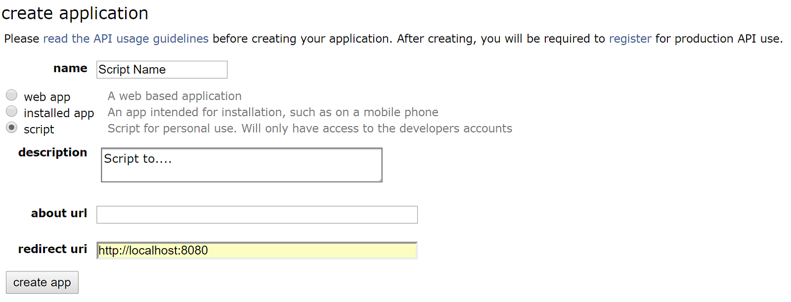 #
# 6. Hit the create app button once you have populated all fields. You should now have a script which resembles the following:
#
#
#
# 6. Hit the create app button once you have populated all fields. You should now have a script which resembles the following:
#
# 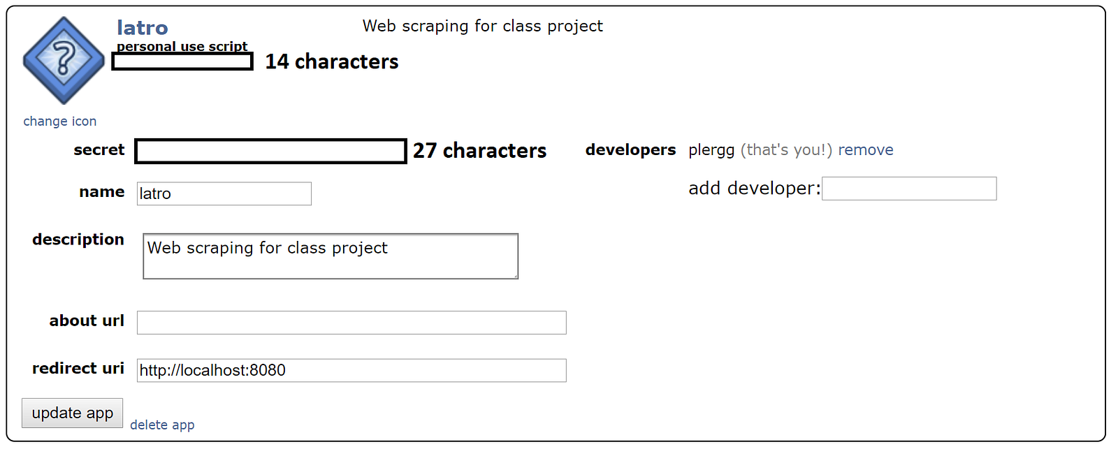 #
#
# NOTE: Certain components of the `reddit = praw.Reddit("BasyesianMethodsForHackers")` code have been intentionally omitted. This is because praw requires a user ID for accessing Reddit. the praw function follows the following format:
# ```python
# reddit = praw.Reddit(client_id='PERSONAL_USE_SCRIPT_14_CHARS', \
# client_secret='SECRET_KEY_27_CHARS ', \
# user_agent='YOUR_APP_NAME', \
# username='YOUR_REDDIT_USER_NAME', \
# password='YOUR_REDDIT_LOGIN_PASSWORD')
# ```
# For help with creating a Reddit instance, visit
# https://praw.readthedocs.io/en/latest/code_overview/reddit_instance.html.
#
# For help on configuring PRAW, visit
# https://praw.readthedocs.io/en/latest/getting_started/configuration.html.
# In[9]:
#@title Reddit API setup
import sys
import numpy as np
from IPython.core.display import Image
import praw
reset_sess()
enter_client_id = 'ZhGqHeR1zTM9fg' #@param {type:"string"}
enter_client_secret = 'keZdvIa1Ge257NKEm3v-eGEdv8M' #@param {type:"string"}
enter_user_agent = "bayesian_app" #@param {type:"string"}
enter_username = "ThisIsJustADemo" #@param {type:"string"}
enter_password = "EnterYourOwnInfoHere" #@param {type:"string"}
subreddit_name = "showerthoughts" #@param ["showerthoughts", "todayilearned", "worldnews", "science", "lifeprotips", "nottheonion"] {allow-input: true}
reddit = praw.Reddit(client_id=enter_client_id,
client_secret=enter_client_secret,
user_agent=enter_user_agent,
username=enter_username,
password=enter_password)
subreddit = reddit.subreddit(subreddit_name)
# go by timespan - 'hour', 'day', 'week', 'month', 'year', 'all'
# might need to go longer than an hour to get entries...
timespan = 'day' #@param ['hour', 'day', 'week', 'month', 'year', 'all']
top_submissions = subreddit.top(timespan)
#adding a number to the inside of int() call will get the ith top post.
ith_top_post = 2 #@param {type:"number"}
n_sub = int(ith_top_post)
i = 0
while i < n_sub:
top_submission = next(top_submissions)
i += 1
top_post = top_submission.title
upvotes = []
downvotes = []
contents = []
for sub in top_submissions:
try:
ratio = sub.upvote_ratio
ups = int(round((ratio*sub.score)/(2*ratio - 1))
if ratio != 0.5 else round(sub.score/2))
upvotes.append(ups)
downvotes.append(ups - sub.score)
contents.append(sub.title)
except Exception as e:
continue
votes = np.array( [ upvotes, downvotes] ).T
print("Post contents: \n")
print(top_post)
# Above is the top post as well as some other sample posts:
# In[10]:
"""
contents: an array of the text from the last 100 top submissions to a subreddit
votes: a 2d numpy array of upvotes, downvotes for each submission.
"""
n_submissions_ = len(votes)
submissions = tfd.Uniform(low=float(0.), high=float(n_submissions_)).sample(sample_shape=(4))
submissions_ = evaluate(tf.cast(submissions,tf.int32))
print("Some Submissions (out of %d total) \n-----------"%n_submissions_)
for i in submissions_:
print('"' + contents[i] + '"')
print("upvotes/downvotes: ",votes[i,:], "\n")
# For a given true upvote ratio $p$ and $N$ votes, the number of upvotes will look like a Binomial random variable with parameters $p$ and $N$. (This is because of the equivalence between upvote ratio and probability of upvoting versus downvoting, out of $N$ possible votes/trials). We create a function that performs Bayesian inference on $p$, for a particular submission's upvote/downvote pair.
# In[ ]:
def joint_log_prob(upvotes, N, test_upvote_ratio):
"""
Args:
upvotes: observed upvotes for a submission
N : observed upvotes+downvotes for the submission
test_upvote_ratio: hypothesized value for true value of upvote ratio
Returns:
Joint log probability optimization function to compute true upvote ratio.
"""
tfd = tfp.distributions
# use a uniform prior
rv_upvote_ratio = tfd.Uniform(name="upvote_ratio", low=0., high=1.)
rv_observations = tfd.Binomial(name="obs",
total_count=float(N),
probs=test_upvote_ratio)
return (
rv_upvote_ratio.log_prob(test_upvote_ratio)
+ rv_observations.log_prob(float(upvotes))
)
# in some cases we might want to run someting like an HMC for multiple, or a variable number, of inputs. Loops are common examples of this. Here we define our function for setting up an HMC that can take in different numbers of upvotes and/or downvotes.
# In[ ]:
def posterior_upvote_ratio(upvotes, downvotes):
reset_sess()
burnin = 5000
N = float(upvotes) + float(downvotes)
# Initialize the step_size. (It will be automatically adapted.)
with tf.variable_scope(tf.get_variable_scope(), reuse=tf.AUTO_REUSE):
step_size = tf.get_variable(
name='step_size',
initializer=tf.constant(0.5, dtype=tf.float32),
trainable=False,
use_resource=True
)
# Set the chain's start state.
initial_chain_state = [
0.5 * tf.ones([], dtype=tf.float32, name="init_upvote_ratio")
]
# Since HMC operates over unconstrained space, we need to transform the
# samples so they live in real-space.
unconstraining_bijectors = [
tfp.bijectors.Sigmoid()
]
# Define a closure over our joint_log_prob.
unnormalized_posterior_log_prob = lambda *args: joint_log_prob(upvotes, N, *args)
hmc=tfp.mcmc.TransformedTransitionKernel(
inner_kernel=tfp.mcmc.HamiltonianMonteCarlo(
target_log_prob_fn=unnormalized_posterior_log_prob,
num_leapfrog_steps=2,
step_size=step_size,
state_gradients_are_stopped=True),
bijector=unconstraining_bijectors)
hmc = tfp.mcmc.SimpleStepSizeAdaptation(
inner_kernel=hmc, num_adaptation_steps=int(burnin * 0.8)
)
# Sample from the chain.
[
posterior_upvote_ratio
], kernel_results = tfp.mcmc.sample_chain(
num_results=20000,
num_burnin_steps=burnin,
current_state=initial_chain_state,
kernel=hmc)
# Initialize any created variables.
init_g = tf.global_variables_initializer()
init_l = tf.local_variables_initializer()
evaluate(init_g)
evaluate(init_l)
return evaluate([
posterior_upvote_ratio,
kernel_results,
])
# In[13]:
plt.figure(figsize(11., 8))
posteriors = []
colours = ["#5DA5DA", "#F15854", "#B276B2", "#60BD68", "#F17CB0"]
for i in range(len(submissions_)):
j = submissions_[i]
posteriors.append( posterior_upvote_ratio(votes[j, 0], votes[j, 1])[0] )
plt.hist( posteriors[i], bins = 10, normed = True, alpha = .9,
histtype="step",color = colours[i], lw = 3,
label = '(%d up:%d down)\n%s...'%(votes[j, 0], votes[j,1], contents[j][:50]) )
plt.hist( posteriors[i], bins = 10, normed = True, alpha = .2,
histtype="stepfilled",color = colours[i], lw = 3, )
plt.legend(loc="upper left")
plt.xlim( 0, 1)
plt.title("Posterior distributions of upvote ratios on different submissions");
# Some distributions are very tight, others have very long tails (relatively speaking), expressing our uncertainty with what the true upvote ratio might be.
#
# #### Sorting!
#
# We have been ignoring the goal of this exercise: how do we sort the submissions from *best to worst*? Of course, we cannot sort distributions, we must sort scalar numbers. There are many ways to distill a distribution down to a scalar: expressing the distribution through its expected value, or mean, is one way. Choosing the mean is a bad choice though. This is because the mean does not take into account the uncertainty of distributions.
#
# I suggest using the *95% least plausible value*, defined as the value such that there is only a 5% chance the true parameter is lower (think of the lower bound on the 95% credible region). Below are the posterior distributions with the 95% least-plausible value plotted:
# In[14]:
N = posteriors[0].shape[0]
lower_limits = []
for i in range(len(submissions_)):
j = submissions_[i]
plt.hist( posteriors[i], bins = 20, normed = True, alpha = .9,
histtype="step",color = colours[i], lw = 3,
label = '(%d up:%d down)\n%s...'%(votes[j, 0], votes[j,1], contents[j][:50]) )
plt.hist( posteriors[i], bins = 20, normed = True, alpha = .2,
histtype="stepfilled",color = colours[i], lw = 3, )
v = np.sort( posteriors[i] )[ int(0.05*N) ]
plt.vlines( v, 0, 30 , color = colours[i], linestyles = "--", linewidths=3 )
lower_limits.append(v)
plt.legend(loc="upper left")
plt.legend(loc="upper left")
plt.title("Posterior distributions of upvote ratios on different submissions");
order = np.argsort( -np.array( lower_limits ) )
print(order, lower_limits)
# The best submissions, according to our procedure, are the submissions that are *most-likely* to score a high percentage of upvotes. Visually those are the submissions with the 95% least plausible value close to 1.
#
# Why is sorting based on this quantity a good idea? By ordering by the 95% least plausible value, we are being the most conservative with what we think is best. When using the lower-bound of the 95% credible interval, we believe with high certainty that the 'true upvote ratio' is at the very least equal to this value (or greater), thereby ensuring that the best submissions are still on top. Under this ordering, we impose the following very natural properties:
#
# 1. given two submissions with the same observed upvote ratio, we will assign the submission with more votes as better (since we are more confident it has a higher ratio).
# 2. given two submissions with the same number of votes, we still assign the submission with more upvotes as *better*.
#
# #### But this is too slow for real-time!
#
# I agree, computing the posterior of every submission takes a long time, and by the time you have computed it, likely the data has changed. I delay the mathematics to the appendix, but I suggest using the following formula to compute the lower bound very fast.
#
# $$ \frac{a}{a + b} - 1.65\sqrt{ \frac{ab}{ (a+b)^2(a + b +1 ) } }$$
#
# where
# $$
# \begin{align}
# & a = 1 + u \\
# & b = 1 + d \\
# \end{align}
# $$
# $u$ is the number of upvotes, and $d$ is the number of downvotes. The formula is a shortcut in Bayesian inference, which will be further explained in Chapter 6 when we discuss priors in more detail.
# In[15]:
def intervals(u, d):
a = tf.add(1., u)
b = tf.add(1., d)
mu = tf.divide(x=a, y=tf.add(1., u))
std_err = 1.65 * tf.sqrt((a * b) / ((a + b) ** 2 * (a + b + 1.)))
return (mu, std_err)
print("Approximate lower bounds:")
posterior_mean, std_err = evaluate(intervals(votes[:,0],votes[:,1]))
lb = posterior_mean - std_err
print(lb)
print("\n")
print("Top 40 Sorted according to approximate lower bounds:")
print("\n")
[ order ] = evaluate([tf.nn.top_k(lb, k=lb.shape[0], sorted=True)])
ordered_contents = []
for i, N in enumerate(order.values[:40]):
ordered_contents.append( contents[i] )
print(votes[i,0], votes[i,1], contents[i])
print("-------------")
# We can view the ordering visually by plotting the posterior mean and bounds, and sorting by the lower bound. In the plot below, notice that the left error-bar is sorted (as we suggested this is the best way to determine an ordering), so the means, indicated by dots, do not follow any strong pattern.
# In[16]:
r_order = order.indices[::-1][-40:]
ratio_range_ = evaluate(tf.range( len(r_order)-1,-1,-1 ))
r_order_vals = order.values[::-1][-40:]
plt.errorbar( r_order_vals,
np.arange( len(r_order) ),
xerr=std_err[r_order], capsize=0, fmt="o",
color = TFColor[0])
plt.xlim( 0.3, 1)
plt.yticks( ratio_range_ , map( lambda x: x[:30].replace("\n",""), ordered_contents) );
# In the graphic above, you can see why sorting by mean would be sub-optimal.
# ### Extension to Starred rating systems
#
# The above procedure works well for upvote-downvotes schemes, but what about systems that use star ratings, e.g. 5 star rating systems. Similar problems apply with simply taking the average: an item with two perfect ratings would beat an item with thousands of perfect ratings, but a single sub-perfect rating.
#
#
# We can consider the upvote-downvote problem above as binary: 0 is a downvote, 1 if an upvote. A $N$-star rating system can be seen as a more continuous version of above, and we can set $n$ stars rewarded is equivalent to rewarding $\frac{n}{N}$. For example, in a 5-star system, a 2 star rating corresponds to 0.4. A perfect rating is a 1. We can use the same formula as before, but with $a,b$ defined differently:
#
#
# $$ \frac{a}{a + b} - 1.65\sqrt{ \frac{ab}{ (a+b)^2(a + b +1 ) } }$$
#
# where
# $$
# \begin{align}
# & a = 1 + S \\
# & b = 1 + N - S \\
# \end{align}
# $$
# where $N$ is the number of users who rated, and $S$ is the sum of all the ratings, under the equivalence scheme mentioned above.
# ### Example: Counting Github stars
#
# What is the average number of stars a Github repository has? How would you calculate this? There are over 6 million respositories, so there is more than enough data to invoke the Law of Large numbers. Let's start pulling some data.
# In[17]:
reset_sess()
import wget
url = 'https://raw.githubusercontent.com/CamDavidsonPilon/Probabilistic-Programming-and-Bayesian-Methods-for-Hackers/master/Chapter3_MCMC/data/github_data.csv'
filename = wget.download(url)
filename
# In[18]:
# Github data scrapper
# See documentation_url: https://developer.github.com/v3/
from json import loads
import datetime
import numpy as np
from requests import get
"""
variables of interest:
indp. variables
- language, given as a binary variable. Need 4 positions for 5 langagues
- #number of days created ago, 1 position
- has wiki? Boolean, 1 position
- followers, 1 position
- following, 1 position
- constant
dep. variables
-stars/watchers
-forks
"""
MAX = 8000000
today = datetime.datetime.today()
randint = np.random.randint
N = 20 #sample size.
auth = ("mikeshwe", "kick#Ass1" )
language_mappings = {"Python": 0, "JavaScript": 1, "Ruby": 2, "Java":3, "Shell":4, "PHP":5}
#define data matrix:
X = np.zeros( (N , 12), dtype = int )
for i in range(N):
is_fork = True
is_valid_language = False
while is_fork == True or is_valid_language == False:
is_fork = True
is_valid_language = False
params = {"since":randint(0, MAX ) }
r = get("https://api.github.com/repositories", params = params, auth=auth )
results = loads( r.text )[0]
#im only interested in the first one, and if it is not a fork.
#print(results)
is_fork = results["fork"]
r = get( results["url"], auth = auth)
#check the language
repo_results = loads( r.text )
try:
language_mappings[ repo_results["language" ] ]
is_valid_language = True
except:
pass
#languages
X[ i, language_mappings[ repo_results["language" ] ] ] = 1
#delta time
X[ i, 6] = ( today - datetime.datetime.strptime( repo_results["created_at"][:10], "%Y-%m-%d" ) ).days
#haswiki
X[i, 7] = repo_results["has_wiki"]
#get user information
r = get( results["owner"]["url"] , auth = auth)
user_results = loads( r.text )
X[i, 8] = user_results["following"]
X[i, 9] = user_results["followers"]
#get dep. data
X[i, 10] = repo_results["watchers_count"]
X[i, 11] = repo_results["forks_count"]
print()
print(" -------------- ")
print(i, ": ", results["full_name"], repo_results["language" ], repo_results["watchers_count"], repo_results["forks_count"])
print(" -------------- ")
print()
np.savetxt("github_data.csv", X, delimiter=",", fmt="%d" )
# ### Conclusion
#
# While the Law of Large Numbers is cool, it is only true so much as its name implies: with large sample sizes only. We have seen how our inference can be affected by not considering *how the data is shaped*.
#
# 1. By (cheaply) drawing many samples from the posterior distributions, we can ensure that the Law of Large Number applies as we approximate expected values (which we will do in the next chapter).
#
# 2. Bayesian inference understands that with small sample sizes, we can observe wild randomness. Our posterior distribution will reflect this by being more spread rather than tightly concentrated. Thus, our inference should be correctable.
#
# 3. There are major implications of not considering the sample size, and trying to sort objects that are unstable leads to pathological orderings. The method provided above solves this problem.
#
# ### Appendix
#
# ##### Derivation of sorting submissions formula
#
# Basically what we are doing is using a Beta prior (with parameters $a=1, b=1$, which is a uniform distribution), and using a Binomial likelihood with observations $u, N = u+d$. This means our posterior is a Beta distribution with parameters $a' = 1 + u, b' = 1 + (N - u) = 1+d$. We then need to find the value, $x$, such that 0.05 probability is less than $x$. This is usually done by inverting the CDF ([Cumulative Distribution Function](http://en.wikipedia.org/wiki/Cumulative_Distribution_Function)), but the CDF of the beta, for integer parameters, is known but is a large sum [3].
#
# We instead use a Normal approximation. The mean of the Beta is $\mu = a'/(a'+b')$ and the variance is
#
# $$\sigma^2 = \frac{a'b'}{ (a' + b')^2(a'+b'+1) }$$
#
# Hence we solve the following equation for $x$ and have an approximate lower bound.
#
# $$ 0.05 = \Phi\left( \frac{(x - \mu)}{\sigma}\right) $$
#
# $\Phi$ being the [cumulative distribution for the normal distribution](http://en.wikipedia.org/wiki/Normal_distribution#Cumulative_distribution)
# ##### Exercises
#
# 1\. How would you estimate the quantity $E\left[ \cos{X} \right]$, where $X \sim \text{Exp}(4)$? What about $E\left[ \cos{X} | X \lt 1\right]$, i.e. the expected value *given* we know $X$ is less than 1? Would you need more samples than the original samples size to be equally accurate?
# In[19]:
## Enter code here
get_ipython().run_line_magic('%time', '')
import tensorflow as tf
import tensorflow_probability as tfp
tfd = tf.distributions
exp = tfd.Exponential(rate=4.)
N = 10000
X = exp.sample(sample_shape=int(N))
with tf.Session() as exercise_1:
print(X.eval())
## ...
# 2\. The following table was located in the paper "Going for Three: Predicting the Likelihood of Field Goal Success with Logistic Regression" [2]. The table ranks football field-goal kickers by their percent of non-misses. What mistake have the researchers made?
#
# -----
#
# #### Kicker Careers Ranked by Make Percentage
#
#
#
# NOTE: Certain components of the `reddit = praw.Reddit("BasyesianMethodsForHackers")` code have been intentionally omitted. This is because praw requires a user ID for accessing Reddit. the praw function follows the following format:
# ```python
# reddit = praw.Reddit(client_id='PERSONAL_USE_SCRIPT_14_CHARS', \
# client_secret='SECRET_KEY_27_CHARS ', \
# user_agent='YOUR_APP_NAME', \
# username='YOUR_REDDIT_USER_NAME', \
# password='YOUR_REDDIT_LOGIN_PASSWORD')
# ```
# For help with creating a Reddit instance, visit
# https://praw.readthedocs.io/en/latest/code_overview/reddit_instance.html.
#
# For help on configuring PRAW, visit
# https://praw.readthedocs.io/en/latest/getting_started/configuration.html.
# In[9]:
#@title Reddit API setup
import sys
import numpy as np
from IPython.core.display import Image
import praw
reset_sess()
enter_client_id = 'ZhGqHeR1zTM9fg' #@param {type:"string"}
enter_client_secret = 'keZdvIa1Ge257NKEm3v-eGEdv8M' #@param {type:"string"}
enter_user_agent = "bayesian_app" #@param {type:"string"}
enter_username = "ThisIsJustADemo" #@param {type:"string"}
enter_password = "EnterYourOwnInfoHere" #@param {type:"string"}
subreddit_name = "showerthoughts" #@param ["showerthoughts", "todayilearned", "worldnews", "science", "lifeprotips", "nottheonion"] {allow-input: true}
reddit = praw.Reddit(client_id=enter_client_id,
client_secret=enter_client_secret,
user_agent=enter_user_agent,
username=enter_username,
password=enter_password)
subreddit = reddit.subreddit(subreddit_name)
# go by timespan - 'hour', 'day', 'week', 'month', 'year', 'all'
# might need to go longer than an hour to get entries...
timespan = 'day' #@param ['hour', 'day', 'week', 'month', 'year', 'all']
top_submissions = subreddit.top(timespan)
#adding a number to the inside of int() call will get the ith top post.
ith_top_post = 2 #@param {type:"number"}
n_sub = int(ith_top_post)
i = 0
while i < n_sub:
top_submission = next(top_submissions)
i += 1
top_post = top_submission.title
upvotes = []
downvotes = []
contents = []
for sub in top_submissions:
try:
ratio = sub.upvote_ratio
ups = int(round((ratio*sub.score)/(2*ratio - 1))
if ratio != 0.5 else round(sub.score/2))
upvotes.append(ups)
downvotes.append(ups - sub.score)
contents.append(sub.title)
except Exception as e:
continue
votes = np.array( [ upvotes, downvotes] ).T
print("Post contents: \n")
print(top_post)
# Above is the top post as well as some other sample posts:
# In[10]:
"""
contents: an array of the text from the last 100 top submissions to a subreddit
votes: a 2d numpy array of upvotes, downvotes for each submission.
"""
n_submissions_ = len(votes)
submissions = tfd.Uniform(low=float(0.), high=float(n_submissions_)).sample(sample_shape=(4))
submissions_ = evaluate(tf.cast(submissions,tf.int32))
print("Some Submissions (out of %d total) \n-----------"%n_submissions_)
for i in submissions_:
print('"' + contents[i] + '"')
print("upvotes/downvotes: ",votes[i,:], "\n")
# For a given true upvote ratio $p$ and $N$ votes, the number of upvotes will look like a Binomial random variable with parameters $p$ and $N$. (This is because of the equivalence between upvote ratio and probability of upvoting versus downvoting, out of $N$ possible votes/trials). We create a function that performs Bayesian inference on $p$, for a particular submission's upvote/downvote pair.
# In[ ]:
def joint_log_prob(upvotes, N, test_upvote_ratio):
"""
Args:
upvotes: observed upvotes for a submission
N : observed upvotes+downvotes for the submission
test_upvote_ratio: hypothesized value for true value of upvote ratio
Returns:
Joint log probability optimization function to compute true upvote ratio.
"""
tfd = tfp.distributions
# use a uniform prior
rv_upvote_ratio = tfd.Uniform(name="upvote_ratio", low=0., high=1.)
rv_observations = tfd.Binomial(name="obs",
total_count=float(N),
probs=test_upvote_ratio)
return (
rv_upvote_ratio.log_prob(test_upvote_ratio)
+ rv_observations.log_prob(float(upvotes))
)
# in some cases we might want to run someting like an HMC for multiple, or a variable number, of inputs. Loops are common examples of this. Here we define our function for setting up an HMC that can take in different numbers of upvotes and/or downvotes.
# In[ ]:
def posterior_upvote_ratio(upvotes, downvotes):
reset_sess()
burnin = 5000
N = float(upvotes) + float(downvotes)
# Initialize the step_size. (It will be automatically adapted.)
with tf.variable_scope(tf.get_variable_scope(), reuse=tf.AUTO_REUSE):
step_size = tf.get_variable(
name='step_size',
initializer=tf.constant(0.5, dtype=tf.float32),
trainable=False,
use_resource=True
)
# Set the chain's start state.
initial_chain_state = [
0.5 * tf.ones([], dtype=tf.float32, name="init_upvote_ratio")
]
# Since HMC operates over unconstrained space, we need to transform the
# samples so they live in real-space.
unconstraining_bijectors = [
tfp.bijectors.Sigmoid()
]
# Define a closure over our joint_log_prob.
unnormalized_posterior_log_prob = lambda *args: joint_log_prob(upvotes, N, *args)
hmc=tfp.mcmc.TransformedTransitionKernel(
inner_kernel=tfp.mcmc.HamiltonianMonteCarlo(
target_log_prob_fn=unnormalized_posterior_log_prob,
num_leapfrog_steps=2,
step_size=step_size,
state_gradients_are_stopped=True),
bijector=unconstraining_bijectors)
hmc = tfp.mcmc.SimpleStepSizeAdaptation(
inner_kernel=hmc, num_adaptation_steps=int(burnin * 0.8)
)
# Sample from the chain.
[
posterior_upvote_ratio
], kernel_results = tfp.mcmc.sample_chain(
num_results=20000,
num_burnin_steps=burnin,
current_state=initial_chain_state,
kernel=hmc)
# Initialize any created variables.
init_g = tf.global_variables_initializer()
init_l = tf.local_variables_initializer()
evaluate(init_g)
evaluate(init_l)
return evaluate([
posterior_upvote_ratio,
kernel_results,
])
# In[13]:
plt.figure(figsize(11., 8))
posteriors = []
colours = ["#5DA5DA", "#F15854", "#B276B2", "#60BD68", "#F17CB0"]
for i in range(len(submissions_)):
j = submissions_[i]
posteriors.append( posterior_upvote_ratio(votes[j, 0], votes[j, 1])[0] )
plt.hist( posteriors[i], bins = 10, normed = True, alpha = .9,
histtype="step",color = colours[i], lw = 3,
label = '(%d up:%d down)\n%s...'%(votes[j, 0], votes[j,1], contents[j][:50]) )
plt.hist( posteriors[i], bins = 10, normed = True, alpha = .2,
histtype="stepfilled",color = colours[i], lw = 3, )
plt.legend(loc="upper left")
plt.xlim( 0, 1)
plt.title("Posterior distributions of upvote ratios on different submissions");
# Some distributions are very tight, others have very long tails (relatively speaking), expressing our uncertainty with what the true upvote ratio might be.
#
# #### Sorting!
#
# We have been ignoring the goal of this exercise: how do we sort the submissions from *best to worst*? Of course, we cannot sort distributions, we must sort scalar numbers. There are many ways to distill a distribution down to a scalar: expressing the distribution through its expected value, or mean, is one way. Choosing the mean is a bad choice though. This is because the mean does not take into account the uncertainty of distributions.
#
# I suggest using the *95% least plausible value*, defined as the value such that there is only a 5% chance the true parameter is lower (think of the lower bound on the 95% credible region). Below are the posterior distributions with the 95% least-plausible value plotted:
# In[14]:
N = posteriors[0].shape[0]
lower_limits = []
for i in range(len(submissions_)):
j = submissions_[i]
plt.hist( posteriors[i], bins = 20, normed = True, alpha = .9,
histtype="step",color = colours[i], lw = 3,
label = '(%d up:%d down)\n%s...'%(votes[j, 0], votes[j,1], contents[j][:50]) )
plt.hist( posteriors[i], bins = 20, normed = True, alpha = .2,
histtype="stepfilled",color = colours[i], lw = 3, )
v = np.sort( posteriors[i] )[ int(0.05*N) ]
plt.vlines( v, 0, 30 , color = colours[i], linestyles = "--", linewidths=3 )
lower_limits.append(v)
plt.legend(loc="upper left")
plt.legend(loc="upper left")
plt.title("Posterior distributions of upvote ratios on different submissions");
order = np.argsort( -np.array( lower_limits ) )
print(order, lower_limits)
# The best submissions, according to our procedure, are the submissions that are *most-likely* to score a high percentage of upvotes. Visually those are the submissions with the 95% least plausible value close to 1.
#
# Why is sorting based on this quantity a good idea? By ordering by the 95% least plausible value, we are being the most conservative with what we think is best. When using the lower-bound of the 95% credible interval, we believe with high certainty that the 'true upvote ratio' is at the very least equal to this value (or greater), thereby ensuring that the best submissions are still on top. Under this ordering, we impose the following very natural properties:
#
# 1. given two submissions with the same observed upvote ratio, we will assign the submission with more votes as better (since we are more confident it has a higher ratio).
# 2. given two submissions with the same number of votes, we still assign the submission with more upvotes as *better*.
#
# #### But this is too slow for real-time!
#
# I agree, computing the posterior of every submission takes a long time, and by the time you have computed it, likely the data has changed. I delay the mathematics to the appendix, but I suggest using the following formula to compute the lower bound very fast.
#
# $$ \frac{a}{a + b} - 1.65\sqrt{ \frac{ab}{ (a+b)^2(a + b +1 ) } }$$
#
# where
# $$
# \begin{align}
# & a = 1 + u \\
# & b = 1 + d \\
# \end{align}
# $$
# $u$ is the number of upvotes, and $d$ is the number of downvotes. The formula is a shortcut in Bayesian inference, which will be further explained in Chapter 6 when we discuss priors in more detail.
# In[15]:
def intervals(u, d):
a = tf.add(1., u)
b = tf.add(1., d)
mu = tf.divide(x=a, y=tf.add(1., u))
std_err = 1.65 * tf.sqrt((a * b) / ((a + b) ** 2 * (a + b + 1.)))
return (mu, std_err)
print("Approximate lower bounds:")
posterior_mean, std_err = evaluate(intervals(votes[:,0],votes[:,1]))
lb = posterior_mean - std_err
print(lb)
print("\n")
print("Top 40 Sorted according to approximate lower bounds:")
print("\n")
[ order ] = evaluate([tf.nn.top_k(lb, k=lb.shape[0], sorted=True)])
ordered_contents = []
for i, N in enumerate(order.values[:40]):
ordered_contents.append( contents[i] )
print(votes[i,0], votes[i,1], contents[i])
print("-------------")
# We can view the ordering visually by plotting the posterior mean and bounds, and sorting by the lower bound. In the plot below, notice that the left error-bar is sorted (as we suggested this is the best way to determine an ordering), so the means, indicated by dots, do not follow any strong pattern.
# In[16]:
r_order = order.indices[::-1][-40:]
ratio_range_ = evaluate(tf.range( len(r_order)-1,-1,-1 ))
r_order_vals = order.values[::-1][-40:]
plt.errorbar( r_order_vals,
np.arange( len(r_order) ),
xerr=std_err[r_order], capsize=0, fmt="o",
color = TFColor[0])
plt.xlim( 0.3, 1)
plt.yticks( ratio_range_ , map( lambda x: x[:30].replace("\n",""), ordered_contents) );
# In the graphic above, you can see why sorting by mean would be sub-optimal.
# ### Extension to Starred rating systems
#
# The above procedure works well for upvote-downvotes schemes, but what about systems that use star ratings, e.g. 5 star rating systems. Similar problems apply with simply taking the average: an item with two perfect ratings would beat an item with thousands of perfect ratings, but a single sub-perfect rating.
#
#
# We can consider the upvote-downvote problem above as binary: 0 is a downvote, 1 if an upvote. A $N$-star rating system can be seen as a more continuous version of above, and we can set $n$ stars rewarded is equivalent to rewarding $\frac{n}{N}$. For example, in a 5-star system, a 2 star rating corresponds to 0.4. A perfect rating is a 1. We can use the same formula as before, but with $a,b$ defined differently:
#
#
# $$ \frac{a}{a + b} - 1.65\sqrt{ \frac{ab}{ (a+b)^2(a + b +1 ) } }$$
#
# where
# $$
# \begin{align}
# & a = 1 + S \\
# & b = 1 + N - S \\
# \end{align}
# $$
# where $N$ is the number of users who rated, and $S$ is the sum of all the ratings, under the equivalence scheme mentioned above.
# ### Example: Counting Github stars
#
# What is the average number of stars a Github repository has? How would you calculate this? There are over 6 million respositories, so there is more than enough data to invoke the Law of Large numbers. Let's start pulling some data.
# In[17]:
reset_sess()
import wget
url = 'https://raw.githubusercontent.com/CamDavidsonPilon/Probabilistic-Programming-and-Bayesian-Methods-for-Hackers/master/Chapter3_MCMC/data/github_data.csv'
filename = wget.download(url)
filename
# In[18]:
# Github data scrapper
# See documentation_url: https://developer.github.com/v3/
from json import loads
import datetime
import numpy as np
from requests import get
"""
variables of interest:
indp. variables
- language, given as a binary variable. Need 4 positions for 5 langagues
- #number of days created ago, 1 position
- has wiki? Boolean, 1 position
- followers, 1 position
- following, 1 position
- constant
dep. variables
-stars/watchers
-forks
"""
MAX = 8000000
today = datetime.datetime.today()
randint = np.random.randint
N = 20 #sample size.
auth = ("mikeshwe", "kick#Ass1" )
language_mappings = {"Python": 0, "JavaScript": 1, "Ruby": 2, "Java":3, "Shell":4, "PHP":5}
#define data matrix:
X = np.zeros( (N , 12), dtype = int )
for i in range(N):
is_fork = True
is_valid_language = False
while is_fork == True or is_valid_language == False:
is_fork = True
is_valid_language = False
params = {"since":randint(0, MAX ) }
r = get("https://api.github.com/repositories", params = params, auth=auth )
results = loads( r.text )[0]
#im only interested in the first one, and if it is not a fork.
#print(results)
is_fork = results["fork"]
r = get( results["url"], auth = auth)
#check the language
repo_results = loads( r.text )
try:
language_mappings[ repo_results["language" ] ]
is_valid_language = True
except:
pass
#languages
X[ i, language_mappings[ repo_results["language" ] ] ] = 1
#delta time
X[ i, 6] = ( today - datetime.datetime.strptime( repo_results["created_at"][:10], "%Y-%m-%d" ) ).days
#haswiki
X[i, 7] = repo_results["has_wiki"]
#get user information
r = get( results["owner"]["url"] , auth = auth)
user_results = loads( r.text )
X[i, 8] = user_results["following"]
X[i, 9] = user_results["followers"]
#get dep. data
X[i, 10] = repo_results["watchers_count"]
X[i, 11] = repo_results["forks_count"]
print()
print(" -------------- ")
print(i, ": ", results["full_name"], repo_results["language" ], repo_results["watchers_count"], repo_results["forks_count"])
print(" -------------- ")
print()
np.savetxt("github_data.csv", X, delimiter=",", fmt="%d" )
# ### Conclusion
#
# While the Law of Large Numbers is cool, it is only true so much as its name implies: with large sample sizes only. We have seen how our inference can be affected by not considering *how the data is shaped*.
#
# 1. By (cheaply) drawing many samples from the posterior distributions, we can ensure that the Law of Large Number applies as we approximate expected values (which we will do in the next chapter).
#
# 2. Bayesian inference understands that with small sample sizes, we can observe wild randomness. Our posterior distribution will reflect this by being more spread rather than tightly concentrated. Thus, our inference should be correctable.
#
# 3. There are major implications of not considering the sample size, and trying to sort objects that are unstable leads to pathological orderings. The method provided above solves this problem.
#
# ### Appendix
#
# ##### Derivation of sorting submissions formula
#
# Basically what we are doing is using a Beta prior (with parameters $a=1, b=1$, which is a uniform distribution), and using a Binomial likelihood with observations $u, N = u+d$. This means our posterior is a Beta distribution with parameters $a' = 1 + u, b' = 1 + (N - u) = 1+d$. We then need to find the value, $x$, such that 0.05 probability is less than $x$. This is usually done by inverting the CDF ([Cumulative Distribution Function](http://en.wikipedia.org/wiki/Cumulative_Distribution_Function)), but the CDF of the beta, for integer parameters, is known but is a large sum [3].
#
# We instead use a Normal approximation. The mean of the Beta is $\mu = a'/(a'+b')$ and the variance is
#
# $$\sigma^2 = \frac{a'b'}{ (a' + b')^2(a'+b'+1) }$$
#
# Hence we solve the following equation for $x$ and have an approximate lower bound.
#
# $$ 0.05 = \Phi\left( \frac{(x - \mu)}{\sigma}\right) $$
#
# $\Phi$ being the [cumulative distribution for the normal distribution](http://en.wikipedia.org/wiki/Normal_distribution#Cumulative_distribution)
# ##### Exercises
#
# 1\. How would you estimate the quantity $E\left[ \cos{X} \right]$, where $X \sim \text{Exp}(4)$? What about $E\left[ \cos{X} | X \lt 1\right]$, i.e. the expected value *given* we know $X$ is less than 1? Would you need more samples than the original samples size to be equally accurate?
# In[19]:
## Enter code here
get_ipython().run_line_magic('%time', '')
import tensorflow as tf
import tensorflow_probability as tfp
tfd = tf.distributions
exp = tfd.Exponential(rate=4.)
N = 10000
X = exp.sample(sample_shape=int(N))
with tf.Session() as exercise_1:
print(X.eval())
## ...
# 2\. The following table was located in the paper "Going for Three: Predicting the Likelihood of Field Goal Success with Logistic Regression" [2]. The table ranks football field-goal kickers by their percent of non-misses. What mistake have the researchers made?
#
# -----
#
# #### Kicker Careers Ranked by Make Percentage
#