#!/usr/bin/env python
# coding: utf-8
# # AGC Tools 2022: Columnar Analysis with Coffea
# Authors
# Notebook by: Mat Adamec (UNL)
#
#
# coffea:
#
#  #
#
#
# - Lindsey Gray, Matteo Cremonesi, Bo Jayatilaka, Oliver Gutsche, Nick Smith, Allison Hall, Kevin Pedro, Maria Acosta (FNAL); Andrew Melo (Vanderbilt); Stefano Belforte (INFN); and others
# - In collaboration with IRIS-HEP members: Jim Pivarski (Princeton), Ben Galewsky (NCSA), Mark Neubauer (UIUC)
#
#
# coffea-casa:
#
# - Ken Bloom, Oksana Shadura (UNL); Garhan Attebury, Carl Lundstedt, Derek Weitzel (UNL-HCC); Mátyás Selmeci (UWM); Brian Bockelman (Morgridge Institute)
#
# ## Introduction
# ### What is columnar analysis?
#
# The traditional way of analyzing data in HEP involves the event loop. In this paradigm, we would write an explicit loop to go through every event (and through every field of an event that we wish to make a cut on). This method of analysis is rather bulky in comparison to the columnar approach, which (ideally) has no explicit loops at all! Instead, the fields of our data are treated as arrays and analysis is done by way of numpy-like array operations.
#
# 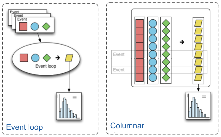 #
# In HEP, numpy is insufficient as our data is non-rectangular (an event can have a variable amount of muons, for example). This problem is resolved by [awkward arrays](https://awkward-array.org/quickstart.html).
# ### What is Coffea?
#
# Awkward arrays let us access data in a columnar fashion, but that's just the first part of doing an analysis. Coffea builds upon this foundation with a variety of features that better enable us to do our analyses. These features include:
#
# * **Hists** give us ROOT-like histograms. Actually, this is now a [standalone package](https://hist.readthedocs.io/en/latest/), but it has been heavily influenced by the (old) coffea hist subpackage, and it's a core component of the coffea ecosystem.
#
# * **NanoEvents** allows us to apply a schema to our awkward array. This schema imposes behavior that we would not have in a simple awkward array, but which makes our (HEP) lives much easier. On one hand, it can serve to better organize our data by providing a structure for naming, nesting, and cross-referencing fields; on the other, it allows us to add physics object methods (e.g., for LorentzVectors).
#
# * **Processors** are coffea's way of encapsulating an analysis in a way that is deployment-neutral. Once you have a Coffea analysis, you can throw it into a processor and use any of a variety of executors (e.g. Dask, Parsl, Spark) to chunk it up and run it across distributed workers. This makes scale-out simple and dynamic for users.
#
# * **Lookup tools** are available in Coffea for any corrections that need to be made to physics data. These tools read a variety of correction file formats and turn them into lookup tables.
#
# In summary, coffea's features enter the analysis pipeline at every step. They improve the usability of our input (NanoEvents), enable us to map it to a histogram output (Hists), and allow us tools for scaling and deployment (Processors).
# ### Looking Ahead
#
# In this tutorial, we will cover some basics of awkward to get a handle on how columnar analysis is done. We will then look at how features of coffea can make our lives easier as we navigate our data and deploy our analysis. By the end, we will seek to plot a Z-peak from our [simulated Z->MuMu dataset](https://opendata.cern.ch/record/21587). It contains approximately 44000 events at 850 MB and is formatted in a generic ntuple format.
#
# An Appendix is placed at the end of this notebook. It contains links to additional resources, as well as for topics which are beyond the scope of this tutorial.
# ### Imports
# In[1]:
# Preliminary
## Columnar analysis basics.
import uproot
import awkward as ak
## Plotting.
import matplotlib.pyplot as plt
# Hists
import hist
from hist import Hist
# NanoEvents
from coffea.nanoevents import NanoEventsFactory, BaseSchema
# Processors
import coffea.processor as processor
# ## **Preliminary**: Columnar Analysis Basics with Awkward
# We begin our tutorial with a crash course through columnar analysis. This is meant to give a basic understanding of columnar operations, but for a more exhaustive introduction to the paradigm itself I recommend referring to an awkward tutorial (refer to the Appendix).
#
# We begin by loading in our data. The standard way to do this is with [uproot](https://uproot.readthedocs.io/en/latest/index.html).
# In[2]:
events = uproot.open('https://xrootd-local.unl.edu:1094//store/user/AGC/zmumu/RunIIFall15MiniAODv2/ZToMuMu_NNPDF30_13TeV-powheg_M_50_120/MINIAODSIM/PU25nsData2015v1_76X_mcRun2_asymptotic_v12-v1/20000/022FAAEA-1BB9-E511-A6DF-44A842CFD5D8.root')['events']
events
# We now have an events tree. We can view its branches by querying its
#
# In HEP, numpy is insufficient as our data is non-rectangular (an event can have a variable amount of muons, for example). This problem is resolved by [awkward arrays](https://awkward-array.org/quickstart.html).
# ### What is Coffea?
#
# Awkward arrays let us access data in a columnar fashion, but that's just the first part of doing an analysis. Coffea builds upon this foundation with a variety of features that better enable us to do our analyses. These features include:
#
# * **Hists** give us ROOT-like histograms. Actually, this is now a [standalone package](https://hist.readthedocs.io/en/latest/), but it has been heavily influenced by the (old) coffea hist subpackage, and it's a core component of the coffea ecosystem.
#
# * **NanoEvents** allows us to apply a schema to our awkward array. This schema imposes behavior that we would not have in a simple awkward array, but which makes our (HEP) lives much easier. On one hand, it can serve to better organize our data by providing a structure for naming, nesting, and cross-referencing fields; on the other, it allows us to add physics object methods (e.g., for LorentzVectors).
#
# * **Processors** are coffea's way of encapsulating an analysis in a way that is deployment-neutral. Once you have a Coffea analysis, you can throw it into a processor and use any of a variety of executors (e.g. Dask, Parsl, Spark) to chunk it up and run it across distributed workers. This makes scale-out simple and dynamic for users.
#
# * **Lookup tools** are available in Coffea for any corrections that need to be made to physics data. These tools read a variety of correction file formats and turn them into lookup tables.
#
# In summary, coffea's features enter the analysis pipeline at every step. They improve the usability of our input (NanoEvents), enable us to map it to a histogram output (Hists), and allow us tools for scaling and deployment (Processors).
# ### Looking Ahead
#
# In this tutorial, we will cover some basics of awkward to get a handle on how columnar analysis is done. We will then look at how features of coffea can make our lives easier as we navigate our data and deploy our analysis. By the end, we will seek to plot a Z-peak from our [simulated Z->MuMu dataset](https://opendata.cern.ch/record/21587). It contains approximately 44000 events at 850 MB and is formatted in a generic ntuple format.
#
# An Appendix is placed at the end of this notebook. It contains links to additional resources, as well as for topics which are beyond the scope of this tutorial.
# ### Imports
# In[1]:
# Preliminary
## Columnar analysis basics.
import uproot
import awkward as ak
## Plotting.
import matplotlib.pyplot as plt
# Hists
import hist
from hist import Hist
# NanoEvents
from coffea.nanoevents import NanoEventsFactory, BaseSchema
# Processors
import coffea.processor as processor
# ## **Preliminary**: Columnar Analysis Basics with Awkward
# We begin our tutorial with a crash course through columnar analysis. This is meant to give a basic understanding of columnar operations, but for a more exhaustive introduction to the paradigm itself I recommend referring to an awkward tutorial (refer to the Appendix).
#
# We begin by loading in our data. The standard way to do this is with [uproot](https://uproot.readthedocs.io/en/latest/index.html).
# In[2]:
events = uproot.open('https://xrootd-local.unl.edu:1094//store/user/AGC/zmumu/RunIIFall15MiniAODv2/ZToMuMu_NNPDF30_13TeV-powheg_M_50_120/MINIAODSIM/PU25nsData2015v1_76X_mcRun2_asymptotic_v12-v1/20000/022FAAEA-1BB9-E511-A6DF-44A842CFD5D8.root')['events']
events
# We now have an events tree. We can view its branches by querying its keys():
# In[3]:
events.keys()
# Each of these branches can be interpreted as an awkward array. Let's examine their contents. Since this is a mumu dataset, it seems natural to look at muons.
# In[4]:
muon_pt = events['muon_pt'].array()
print(muon_pt)
# It's instructive to take a closer look at the structure of this array. First, we see that it is an array of subarrays. Each subarray represents one event, and each element of a subarray represents one muon. It is now clear what we mean by "non-rectangular data." There are a variable amount of muons, so the subarrays are not of equal size.
#
# If we look at another (non-muon) branch, we would expect it to have the same amount of subarrays, but not necessarily the same amount of elements in each subarray. For comparison, let's now look at electrons:
# In[5]:
electron_pt = events['electron_pt'].array()
print(electron_pt)
# In which case it is clear that there are not the same amount of elements in each subarray (most are empty!)
#
# To drive the point home, we can also prove that there is an equal amount of subarrays:
# In[6]:
ak.num(electron_pt, axis=0), ak.num(muon_pt, axis=0)
# A quick note about axes in awkward: 0 is always the shallowest, while -1 is the deepest. In other words, axis=0 would tell us the number of subarrays (events), while axis=-1 would tell us the number of muons within each subarray:
# In[7]:
ak.num(electron_pt, axis=-1), ak.num(muon_pt, axis=-1)
# Then, if we wanted to know the total number of objects (muons or electrons) in our branch, we could just sum up the above output. Given this is a mumu dataset, we'd expect roughly twice as many muons as events and very few electrons. Let's verify this:
# In[8]:
ak.sum(ak.num(electron_pt, axis=-1)), ak.sum(ak.num(muon_pt, axis=-1))
# Okay - so we can access data. How do we actually manipulate it to do analysis? Well, most simple cuts can be handled by masking. A mask is a Boolean array which is generated by applying a condition to a data array. For example, if we want only muons with pT > 10, our mask would be:
# In[9]:
print(muon_pt > 10)
# Then, we can apply the mask to our data. The syntax follows other standard array selection operations: data[mask]. This will pick out only the elements of our data which correspond to a True.
#
# Let's pause and consider the details of this methodology. Our mask in this case must have the same shape as our muons branch, and this is guaranteed to be the case since it is generated from the data in that branch. When we apply this mask, the output should have the same amount of events, but it should down-select muons - muons which correspond to False should be dropped. Let's compare to check:
# In[10]:
print('Input:', muon_pt)
print('Output:', muon_pt[muon_pt > 10])
# We can also confirm we have fewer muons now, but the same amount of events:
# In[11]:
print('Input Counts:', ak.sum(ak.num(muon_pt, axis=1)))
print('Output Counts:', ak.sum(ak.num(muon_pt[muon_pt > 10], axis=1)))
print('Input Size:', ak.num(muon_pt, axis=0))
print('Output Size:', ak.num(muon_pt[ak.num(muon_pt)], axis=0))
# What if we wanted to do a selection on our events, rather than on our muons? Then we'd just need a mask with the same length as our events array, with a True or False entry in place of the subarray instead of the element of the subarray. For example, we might want to select events which have at least one electron. Then our mask would be:
# In[12]:
ak.num(electron_pt) >= 1
# Which you can note does not have the same structure as the muon cut above; it is a flat array. Applying the mask:
# In[13]:
print('Input:', electron_pt)
print('Output:', electron_pt[ak.num(electron_pt) >= 1])
# You can see that the empty arrays have been removed since they don't meet the cut, and the first entry is now the 8.26 we saw in our input. If we look at the size of our input and output arrays now, we will see a discrepency because we have thrown our our empty events:
# In[14]:
print('Input Size:', ak.num(electron_pt, axis=0))
print('Output Size:', ak.num(electron_pt[ak.num(electron_pt) >= 1], axis=0))
# Of course, in this case we still have the same amount of electrons. We've just gotten rid of empty events.
# In[15]:
print('Input Counts:', ak.sum(ak.num(electron_pt, axis=1)))
print('Output Counts:', ak.sum(ak.num(electron_pt[ak.num(electron_pt > 10) >= 1], axis=1)))
# These sorts of cuts are how the bulk of columnar analysis can be done. Awkward comes equipped with features for other standard operations, such as combinatorics and an analogue to np.where() (ak.where()). Other resources (listed in the appendix) cover it more extensively and do it better justice.
#
# Nonetheless, there are a couple of things which aren't exactly pretty. For example, what if we want LorentzVector operations? The nicest way to handle this is with coffea schemas.
# ## **NanoEvents:** Making Data Physics-Friendly
# Before we can dive into our Z-peak analysis, we need to spruce up our data a bit.
#
# Let's turn our attention to NanoEvents and schemas. Schemas let us better organize our file and impose physics methods onto our data. There exist schemas for some standard file formats, most prominently NanoAOD, and there is a BaseSchema which operates much like uproot. The coffea development team welcomes community development of other schemas and it is not so difficult to do so.
#
# For the purposes of this tutorial, I have already made a schema. We won't go into the details, but we will show off its features and the general structure. First, let's take a look at our data structure again. Because there's a lot of branches, we'll zoom in on the muon-related ones here:
# In[16]:
branches = uproot.open("https://xrootd-local.unl.edu:1094//store/user/AGC/zmumu/RunIIFall15MiniAODv2/ZToMuMu_NNPDF30_13TeV-powheg_M_50_120/MINIAODSIM/PU25nsData2015v1_76X_mcRun2_asymptotic_v12-v1/20000/022FAAEA-1BB9-E511-A6DF-44A842CFD5D8.root")['events']
for branch in branches.keys():
if 'muon' in branch:
print(branch)
# By default, uproot (and BaseSchema) treats all of the muon branches as distinct branches with distinct data. This is not ideal, as some of our data is redundant, e.g., all of the nmuon_* branches better have the same counts. Further, we'd expect all the muon_* branches to have the same shape, as each muon should have an entry in each branch.
#
# The first benefit of instating a schema, then, is a standardization of our fields. It would be more succinct to create a general muon collection under which all of these branches (in NanoEvents, fields) with identical size can be housed, and to scrap the redundant ones. We can use numbermuon to figure out how many muons should be in each subarray (the counts, or offsets), and then fill the contents with each muon_* field. We can repeat this for the other branches.
# In[17]:
from agc_schema import AGCSchema
agc_events = NanoEventsFactory.from_root('https://xrootd-local.unl.edu:1094//store/user/AGC/zmumu/RunIIFall15MiniAODv2/ZToMuMu_NNPDF30_13TeV-powheg_M_50_120/MINIAODSIM/PU25nsData2015v1_76X_mcRun2_asymptotic_v12-v1/20000/022FAAEA-1BB9-E511-A6DF-44A842CFD5D8.root', schemaclass=AGCSchema, treepath='events').events()
# For NanoEvents, there is a slightly different syntax to access our data. Instead of querying keys() to find our fields we query fields. We can still access specific fields as we would navigate a dictionary (collection[field]) or we can navigate them in a new way: collection.field.
#
# Let's take a look at our fields now:
# In[18]:
agc_events.fields
# We can confirm that no information has been lost by querying the fields of our event fields:
# In[19]:
agc_events.muon.fields
# All of the branches above are still here, just as fields of our new electron collection. We can confirm this matches our original counts from uproot:
# In[20]:
branches['numbermuon'].array(), ak.num(agc_events.muon)
# So, aesthetically, everything is much nicer. If we had a messier dataset, the schema can also standardize our names to get rid of any quirks. For example, every physics object in our tree has a number{name} field except for GenPart, which has num{name}. This discrepancy is irrelevant after the application of the schema, so we don't have to worry about it.
#
# There are also other benefits to this structure: as we now have a collection object (agc_events.muon), there is a natural place to impose physics methods. By default, this collection object does nothing - it's just a category. But we're physicists, and we often want to deal with Lorentz vectors. Why not treat these objects as such?
#
# This behavior can be built fairly simply into a schema simply by specifying that it is a PtEtaPhiELorentzVector and having the appropriate fields present in each collection (in this case, pt, eta, phi and e). This makes mathematical operations on our muons well-defined:
# In[21]:
agc_events.muon[0, 0] + agc_events.muon[0, 1]
# And it gives us access to all of the standard LorentzVector methods:
# In[22]:
agc_events.muon[0, 0].delta_r(agc_events.muon[0, 1])
# We can also access other LorentzVector formulations, if we want, as the conversions are built-in:
# In[23]:
agc_events.muon.x, agc_events.muon.y, agc_events.muon.z, agc_events.muon.mass
# NanoEvents can also impose other features, such as cross-references in our data; for example, linking the muon jetidx to the jet collection. This is not implemented in our present schema.
# In[24]:
agc_events.muon.fields
# ## **Analysis:** Plotting a Z-Peak
# With an understanding of basic columnar analysis and our data in the proper format, we are finally ready to turn our attention to our analysis. We want to plot the Z-peak. This involves plotting the pair-mass of leptons which have the same flavor (ee or mumu) and opposite sign. To discard anomalies, we also want to toss out leptons with less than 10 pT. This selection is trivial in the columnar paradigm.
#
# A couple of notes: since they're same-flavor, we can consider dimuons and dielectrons independently. Also, since this is a Z -> mumu dataset, we'd only expect to see the Z-peak for muons. There should be few electrons plotted.
# In[25]:
muons = agc_events.muon[agc_events.muon.pt > 10]
electrons = agc_events.electron[agc_events.electron.pt > 10]
dimuons = muons[(ak.num(muons, axis=1) == 2) & (ak.sum(muons.ch, axis=1) == 0)]
dielectrons = electrons[(ak.num(electrons, axis=1) == 2) & (ak.sum(electrons.ch, axis=1) == 0)]
# Our dimuons array should now contain only opposite-charge muon pairs and our dielectrons opposite-charge electron pairs. Let's check!
# In[26]:
dimuons, dielectrons
# Note that the masks performed a cut at the event level rather than the muon level. We have fewer events, but the same amount of leptons in each event (in the events that we kept). That means we've lost the connection between muons and electrons - they've been downselected and it is not the case that the 1st subarray in our electron array is the same event as the 1st subarray in our muon array. This isn't a problem since we're handling the two independently, but there are ways to handle such a selection without downselection if such indexing needs to be preserved.
#
# All we need now is the dilepton mass. Awkward arrays can be indexed in a similar way as numpy arrays, so dimuons[:, 0] will select the first muon in every dimuon event. Recall that NanoEvents allows us to treat mathematical operations on the muon collection level as LorentzVector objects. The same goes for our electrons collection, of course. That makes our life easy:
# In[27]:
mumu_mass = (dimuons[:, 0] + dimuons[:, 1]).mass
ee_mass = (dielectrons[:, 0] + dielectrons[:, 1]).mass
mumu_mass, ee_mass
# This has collapsed our subarrays because we're finding the mass of the pairs, so now we have a flat array. It is of the same size (respectively) as our dimuons and dielectrons arrays above. We now have our data!
#
# What else do we need for plotting? Well, a histogram is essentially a way to reduce our data. We can't just plot every value of dimuon mass, so we divide up our range of masses into n bins across some reasonable range. Thus, we need to define the mapping for our reduction; defining the number of bins and the range is sufficient for this. This is called a Regular axis in the Hist package.
#
# In our case, let's plot 50 bins between values of 0 and 150. This merely cuts off a shrinking tail on the higher end. Because a histogram can contain an arbitrary amount of axes, we also need to give our axis a name (which becomes its reference in our code) and a label (which is the label on the axis that users see when the histogram is plotted).
# In[28]:
ll_bin = hist.axis.Regular(label="Dilepton Mass", name="dilep_mass", bins=50, start=0, stop=150)
# We are still not *yet* ready to plot. We have two masses we'd like to plot, and it doesn't make much sense to throw ee masses into the same bins as $\mu\mu$ masses. We want to keep these separate. We do so by introducing a Categorical axis. Another example of when we might use a categorical axis is to keep data from different datasets separate, though in our case we're only working with a single dataset.
#
# A Categorical axis takes a name, a label, and a pre-defined list of categories.
# In[29]:
ll_cat = hist.axis.StrCategory(label='Leptons', name='lepton', categories=["ee", "$\mu\mu$"])
# We finally have all of the ingredients needed for a histogram! All that remains is to put them together:
# In[30]:
ll_hist = Hist(ll_bin, ll_cat)
# And to fill it with our data:
# In[31]:
ll_hist.fill(lepton="$\mu\mu$", dilep_mass=mumu_mass)
ll_hist.fill(lepton="ee", dilep_mass=ee_mass)
# And plot!
# In[32]:
ll_hist.plot()
plt.legend()
# We can see a peak at around 90 for our dimuon events. Indeed, the mass of a Z boson is ~91.18.
#
# The Hist package is also capable of handling a variety of transormations to our histogram. You should refer to its documentation for more advanced features.
# ## **Processors:** Deploying at Scale
# Now that we have an analysis, we would naturally like to scale it up to a far larger dataset in any practical scenario. More data means more processing time. We try to amend this fact by making use of parallel processing and distributed computing resources, which coffea can be deployed on rather naturally. Importantly, the details of our analysis are entirely independent of our deployment.
#
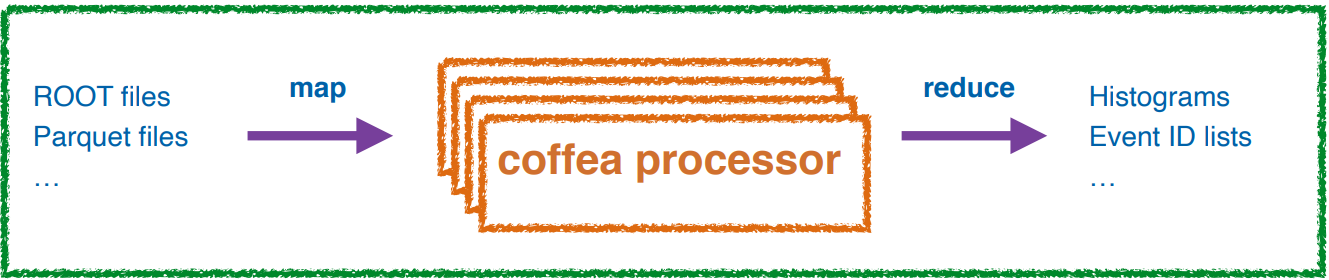
# First, it should be noted that we [b]can[/b] do this in HEP. Events are independent of each other, so if we split our work up and ship it off to different workers, we aren't violating the data's integrity. Furthermore, since the output we seek is a histogram, our output is also independent of how the work is split up. As long as each worker maps its data to a histogram, the summation of those histograms will be identical to a single worker processing all of the data. In coffea, an object that behaves in this way is called an accumulator.
#
# Thus, we have a pipeline: our input data is chunked, sent off to different workers which each execute the processor on their chunk, and then collected and converged once all workers finish processing.
#
# 
#
# We just have to package our analysis in a Processor class.
# In[33]:
import coffea.processor as processor
class Processor(processor.ProcessorABC):
def __init__(self):
pass
def process(self, events):
muons = events.muon[events.muon.pt > 10]
electrons = events.electron[events.electron.pt > 10]
dimuons = muons[(ak.num(muons, axis=1) == 2) & (ak.sum(muons.ch, axis=1) == 0)]
dielectrons = electrons[(ak.num(electrons, axis=1) == 2) & (ak.sum(electrons.ch, axis=1) == 0)]
mumu_mass = (dimuons[:, 0] + dimuons[:, 1]).mass
ee_mass = (dielectrons[:, 0] + dielectrons[:, 1]).mass
ll_bin = hist.axis.Regular(label="Dilepton Mass", name="dilep_mass", bins=50, start=0, stop=150)
ll_cat = hist.axis.StrCategory(label='Leptons', name='lepton', categories=["ee", "$\mu\mu$"])
ll_hist = Hist(ll_bin, ll_cat)
ll_hist.fill(lepton='$\mu\mu$', dilep_mass=mumu_mass)
ll_hist.fill(lepton='ee', dilep_mass=ee_mass)
return ll_hist
def postprocess(self, accumulator):
pass
# To actually deploy our processor, we need to specify an executor. In coffea-casa, we have the ability to tap into Dask, so naturally it is the executor we use. There exist other executors for other big data technologies (e.g., Spark and Parsl), and there also exist executors for local deployment (using Python futures, or just iterating through chunks).
#
# The definition of our executor looks a little blocky. In actuality, it's not too complicated. We have to point to a Dask scheduler (which coordinates workers), and coffea-casa has a scheduler built in at tls://localhost:8786. We need to make sure all of our workers have our schema, since it is a local file, so we upload it through the scheduler. Then we instantiate an executor with our scheduler, apply our schema, and specify how big our chunks should be. Since we only have ~40000 events, we can do a chunk size of 10000.
#
# All that remains is plugging in a file set and specifying the processor we want to run!
# In[34]:
fileset = {'SingleMu' : ['https://xrootd-local.unl.edu:1094//store/user/AGC/zmumu/RunIIFall15MiniAODv2/ZToMuMu_NNPDF30_13TeV-powheg_M_50_120/MINIAODSIM/PU25nsData2015v1_76X_mcRun2_asymptotic_v12-v1/20000/022FAAEA-1BB9-E511-A6DF-44A842CFD5D8.root']}
from dask.distributed import Client
client = Client("tls://localhost:8786")
client.upload_file('agc_schema.py')
run = processor.Runner(executor=processor.DaskExecutor(client=client),
schema=AGCSchema,
chunksize=10000)
output = run(fileset, "events", Processor())
# Where a plot of the output demonstrates the same result as above.
# In[35]:
output.plot()
# Coffea executors also exist with the capabilities to handle other tools within the columnar analysis ecosystem, such as ServiceX, though they are presently a work-in-progress.
# ## Appendix
# ### Coffea
# * [GitHub](https://github.com/CoffeaTeam/coffea)
# * [Documentation and User Guide](https://hist.readthedocs.io/en/latest/)
# * [Tutorials, Sample Analyses, and Other Examples](https://github.com/CoffeaTeam/coffea-casa-tutorials) - see the link's readme for specific details. A good introduction to (progressively) more complicated analysis operations can be found in the [examples](https://github.com/CoffeaTeam/coffea-casa-tutorials/tree/master/examples) folder. A walkthrough for a full-scale analysis can be found in the [tHq analysis](https://github.com/CoffeaTeam/coffea-casa-tutorials/blob/master/analyses/thq/analysis_tutorial.ipynb) folder.
# ### Awkward
# * [GitHub](https://github.com/scikit-hep/awkward-1.0)
# * [Documentation](https://awkward-array.readthedocs.io/en/latest/)
# * [User Guide](https://awkward-array.org/quickstart.html)
# * [Uproot and Awkward Array Tutorial at PyHep 2021](https://github.com/jpivarski-talks/2021-07-06-pyhep-uproot-awkward-tutorial/blob/main/uproot-awkward-tutorial.ipynb)
# ### Hists
# * [GitHub](https://github.com/scikit-hep/hist)
# * [Documentation and User Guide](https://hist.readthedocs.io/en/latest/)
# ### ServiceX (WIP)
# * [Example](https://github.com/iris-hep/analysis-grand-challenge/blob/main/workshops/agctools2021/HZZ_analysis_pipeline/HZZ_analysis_pipeline.ipynb)
# ## Acknowledgements
# These projects are supported by National Science Foundation award 1913513 and OAC-1836650 (through IRIS-HEP).