#!/usr/bin/env python
# coding: utf-8

# <p  style="z-index: 101;background: #fde073;text-align: center;line-height: 2.5;overflow: hidden;font-size:22px;">Please <a href="https://github.com/ECSIM/opem#cite" target="_blank">cite us</a> if you use the software</p>

# #  Chakraborty Dynamic Model

# ### Version 1.4

# <ul>
#     <li><a href="#Overview">Overview</a></li>
#     <li><a href="#Nernst-Voltage">Nernst Voltage</a></li>
#     <ul>
#         <li><a href="#FC-Voltage">FC Voltage</a></li>
#     </ul>
#     <li><a href="#Power-of-PEMFC">Power of PEMFC</a></li>
#     <li><a href="#Efficiency-of-PEMFC">Efficiency of PEMFC</a></li>
#     <li><a href="#Linear-Approximation">Linear Approximation</a></li>
#     <li><a href="#Overall-Parameters">Overall Parameters</a></li>
#     <li><a href="#Full-Run">Full Run</a></li>
#     <li><a href="#Plot">Plot</a></li>
#     <li><a href="#Parameters">Parameters</a></li>
#     <li><a href="#Reference">Reference</a></li>   
# </ul>

# ## Overview

# <p style="text-align:justify;">
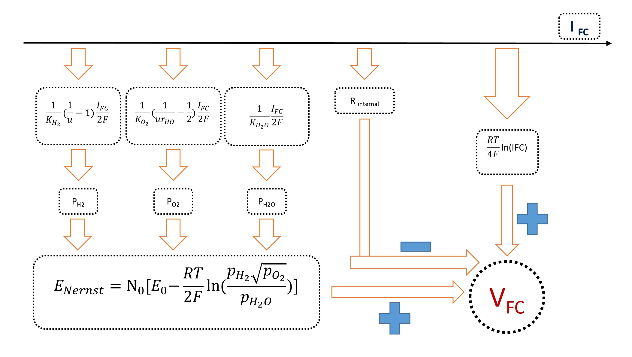
# The new dynamic model is presented based on constant fuel utilization control (constant stoichiometry condition). The model solves the long-standing problem of mixing reversible and irreversible potentials (equilibrium and non-equilibrium states) in the Nernst voltage expression. Specifically, a Nernstian gain term is introduced for the constant fuel utilization condition, and it is shown that the Nernstian gain is an irreversibility in the computation of the output voltage of the fuel cell. 
# </p>

# <div style="text-align:center;">
#     
# <img src="images/Chakraborty-Diagram.jpg" onerror='this.src="../images/Chakraborty-Diagram.jpg"'>  
# <p style="text-align:center;">Fig1. Chakraborty Dynamic Model Block Diagram </p>
#     
# </div>

# ## Nernst Voltage

# $$P_{H_2}=\frac{1}{K_{H_2}}(\frac{1}{u}-1)\frac{i}{2F}$$

# $$P_{O_2}=\frac{1}{K_{O_2}}(\frac{1}{u\times r_{HO}}-\frac{1}{2})\frac{i}{2F}$$

# $$P_{H_2O}=\frac{1}{K_{H_2O}}\frac{i}{2F}$$

# $$E_{Nernst}=N_0\times [E_0-\frac{RT}{2F}ln(\frac{P_{H_2}\times \sqrt{P_{O_2}}}{P_{H_2O}})]$$

# In[1]:


from opem.Dynamic.Chakraborty import PH2_Calc, PO2_Calc, PH2O_Calc, Enernst_Calc


# In[2]:


PH2 = PH2_Calc(KH2=0.000843, u=0.8, I=1)
PO2 = PO2_Calc(KO2=0.00252, u=0.8, rHO=1.145, I=1)
PH2O = PH2O_Calc(KH2O=0.000281, I=1)
Enernst=Enernst_Calc(E0=0.6, N0=1, T=1273, PH2=PH2, PO2=PO2, PH2O=PH2O)
Enernst


# ### FC Voltage

# $$Loss_{Ohmic}=r\times i$$

# $$Gain_{Nernst}=\frac{RT}{4F}ln(i)$$

# $$V_{Fuelcell}=E_{Nernst}+N_0[Gain_{Nernst}-Loss_{Ohmic}]$$

# In[3]:


from opem.Dynamic.Chakraborty import Vcell_Calc, Nernst_Gain_Calc, Ohmic_Loss_Calc


# In[4]:


Ohmic_Loss = Ohmic_Loss_Calc(Rint=3.28125 * 10**(-3) , I=1)


# In[5]:


Nernst_Gain = Nernst_Gain_Calc(T=1273, I=1)


# In[6]:


FC_Voltage=Vcell_Calc(Enernst=Enernst, Nernst_Gain=Nernst_Gain, Ohmic_Loss=Ohmic_Loss, N=1)
FC_Voltage


# ## Power of PEMFC

# $$P=V_{cell}\times i$$

# $$P_{Thermal}=i\times(N \times E_{th}-V_{Stack})$$

# $$E_{th}=\frac{-\Delta H}{nF}=1.23V$$

# In[7]:


from opem.Dynamic.Chakraborty import Power_Calc,Power_Thermal_Calc
Power=Power_Calc(Vcell=FC_Voltage,i=1)
Power


# In[8]:


Power_Thermal_Calc(VStack=FC_Voltage,N=1,i=1)


# ## Efficiency of PEMFC

# $$\eta=\frac{u\times V_{Fuelcell}}{N_0\times HHV}$$

# In[9]:


from opem.Dynamic.Chakraborty import Efficiency_Calc
Efficiency_Calc(Vcell=FC_Voltage,u=0.8,N=1)


# ## Linear Approximation

# Sometimes quick calculations regarding fuel cell efficiency–power-size relationships need to be made. Linear approximation is a good method to find a rough estimate of the value of polarization function at a particular point. A linear polarization curve has the following form:
# $$V_{cell}=V_0-kI$$
# where V0 is the intercept (actual open circuit voltage is always higher) and k is the slope of the curve.
# 
# * Notice : <a href="https://en.wikipedia.org/wiki/Simple_linear_regression">Simple linear regression</a> used for this approximation

# <table style="text-align:center;">
#     <tr>
#         <td>$$Parameter$$</td>
#         <td>$$Description$$</td>
#         <td>$$Unit$$</td>
#     </tr> 
#     <tr>
#         <td>$$V_0$$</td>
#         <td style="text-align:center;">Intercept of the curve obtained by linear approximation</td>
#         <td>$$V$$</td>
#     </tr>
#     <tr>
#         <td>$$k$$</td>
#         <td style="text-align:center;">Slope of the curve obtained by linear approximation</td>
#         <td>$$A^{-1}$$</td>
#     </tr>
#     <tr>
#         <td>$$P_{max}$$</td>
#         <td style="text-align:center;">Maximum power obtained by linear approximation</td>
#         <td>$$W$$</td>
#     </tr>
#     <tr>
#         <td>$$V_{FC}|P_{max}$$</td>
#         <td style="text-align:center;">Cell voltage at maximum power obtained by linear approximation</td>
#         <td>$$V$$</td>
#     </tr>
#    
#      
#     
#     
#     
# </table>

# * Notice : These parameters are only available in HTML report

# ## Overall Parameters

# <table style="text-align:center;">
#     <tr>
#         <td>$$Parameter$$</td>
#         <td>$$Description$$</td>
#         <td>$$Unit$$</td>
#     </tr> 
#     <tr>
#         <td>$$\eta|P_{Max}$$</td>
#         <td style="text-align:center;">Cell efficiency at maximum power</td>
#         <td>$$--$$</td>
#     </tr>
#     <tr>
#         <td>$$P_{Max}$$</td>
#         <td style="text-align:center;">Maximum power </td>
#         <td>$$W$$</td>
#     </tr>
#     <tr>
#         <td>$$P_{Elec} $$</td>
#         <td style="text-align:center;">Total electrical power </td>
#         <td>$$W$$</td>
#     </tr>
#     <tr>
#         <td>$$P_{Thermal} $$</td>
#         <td style="text-align:center;">Total thermal power   </td>
#         <td>$$W$$</td>
#     </tr>
#     <tr>
#         <td>$$V_{FC}|P_{Max}$$</td>
#         <td style="text-align:center;">Cell voltage at maximum power </td>
#         <td>$$V$$</td>
#     </tr>
#    
#      
#     
#     
#     
# </table>

# * Notice : P(Thermal) & P(Elec) calculated by <a href="https://en.wikipedia.org/wiki/Simpson%27s_rule">Simpson's Rule</a>
# 
# * Notice : These parameters are only available in HTML report

# ## Full Run

# * Run from `i`=0.1 to `i`=300 with `step`=0.1

# In[10]:


Test_Vector = {
    "T": 1273,
    "E0": 0.6,
    "u":0.8,
    "N0": 1,
    "R": 3.28125 * 10**(-3),
    "KH2O": 0.000281,
    "KH2": 0.000843,
    "KO2": 0.00252,
    "rho": 1.145,
    "i-start": 0.1,
    "i-stop": 300,
    "i-step": 0.1,
    "Name": "Chakraborty_Test"}


# * Notice : "Name", new in version 0.5

# In[11]:


from opem.Dynamic.Chakraborty import Dynamic_Analysis
data=Dynamic_Analysis(InputMethod=Test_Vector,TestMode=True,PrintMode=True,ReportMode=True)


# In[12]:


data_2=Dynamic_Analysis(InputMethod=Test_Vector,TestMode=True,PrintMode=True,ReportMode=False)


# In[13]:


Dynamic_Analysis(InputMethod={},TestMode=True,PrintMode=False,ReportMode=True)


# ### Parameters

# 1. `TestMode` : Active test mode and get/return data as `dict`, (Default : `False`)
# 2. `ReportMode` : Generate reports(`.csv`,`.opem`,`.html`) and print result in console, (Default : `True`)
# 3. `PrintMode` : Control printing in console, (Default : `True`)
# 4. `Folder` : Reports folder, (Default : `os.getcwd()`)

# * Notice : "Folder" , new in version 1.4

# ## Plot

# In[14]:


import sys
get_ipython().system('{sys.executable} -m pip -qqq install matplotlib;')
import matplotlib.pyplot as plt


# In[15]:


def plot_func(x,y,x_label,y_label,color='green',legend=[],multi=False):
    plt.figure()
    plt.grid()
    if multi==True:
        for index,y_item in enumerate(y):
            plt.plot(x,y_item,color=color[index])
    else:
        plt.plot(x,y,color=color)
    plt.xlabel(x_label)
    plt.ylabel(y_label)
    if len(legend)!=0:
        plt.legend(legend)
    plt.show()


# In[16]:


plot_func(data["I"],data["P"],"I(A)","Power(W)")


# In[17]:


plot_func(data["I"],[data["V"],data["VE"]],"I(A)","V(V)",["red","blue"],legend=["Voltage-Stack","Linear-Apx"],multi=True)


# In[18]:


plot_func(data["I"],[data["Nernst Gain"],data["Ohmic Loss"]],"I(A)","V(V)",["red","blue"],legend=["Nernst Gain","Ohmic Loss"],multi=True)


# In[19]:


plot_func(data["I"],data["Ph"],"I(A)","Power-Thermal(W)","blue")


# In[20]:


plot_func(data["I"],data["EFF"],"I(A)","Efficiency","gray")


# In[21]:


plot_func(data["I"],data["PO2"],"I(A)","PO2(atm)","orange")


# In[22]:


plot_func(data["I"],data["PH2"],"I(A)","PH2(atm)","violet")


# In[23]:


plot_func(data["I"],data["PH2O"],"I(A)","PH2O(atm)","pink")


# <a href="Chakraborty/Chakraborty_Test.html">HTML File</a>

# <a href="Chakraborty/Chakraborty_Test.opem">OPEM File</a>

# <a href="Chakraborty/Chakraborty_Test.csv">CSV File</a>

# ## Parameters

# Inputs, Constants & Middle Values
# 1. User : User input
# 2. System : Simulator calculation (middle value)

# <table style="text-align:center;">
#     <tr>
#         <td>$$Parameter$$</td>
#         <td>$$Description$$</td>
#         <td>$$Unit$$</td>
#         <td>$$Value$$</td>
#     </tr> 
#     <tr>
#         <td>$$E_0$$</td>
#         <td style="text-align:center;">No load voltage</td>
#         <td>$$V$$</td>
#         <td>$$User$$</td>
#     </tr>
#      <tr>
#         <td>$$T$$</td>
#         <td style="text-align:center;">Cell operation temperature</td>
#         <td>$$K$$</td>
#         <td>$$User$$</td>
#     </tr>
#     <tr>
#         <td>$$N_0$$</td>
#         <td style="text-align:center;">Number of cells</td>
#         <td>$$−−$$</td>
#         <td>$$User$$</td>
#     </tr>
#     <tr>
#         <td>$$K_{H_2}$$</td>
#         <td style="text-align:center;">Hydrogen valve constant</td>
#         <td>$$kmol.s^{-1}.atm^{-1}$$</td>
#         <td>$$User$$</td>
#     </tr>
#     <tr>
#         <td>$$K_{H_2O}$$</td>
#         <td style="text-align:center;">Water valve constant</td>
#         <td>$$kmol.s^{-1}.atm^{-1}$$</td>
#         <td>$$User$$</td>
#     </tr>
#     <tr>
#         <td>$$K_{O_2}$$</td>
#         <td style="text-align:center;">Oxygen valve constant</td>
#         <td>$$kmol.s^{-1}.atm^{-1}$$</td>
#         <td>$$User$$</td>
#     </tr>
#     <tr>
#         <td>$$R^{int}$$</td>
#         <td style="text-align:center;">Fuel cell internal resistance</td>
#         <td>$$\Omega$$</td>
#         <td>$$User$$</td>
#     </tr>
#       <tr>
#         <td>$$r_{h-o}$$</td>
#         <td style="text-align:center;">Hydrogen-Oxygen flow ratio</td>
#         <td>$$--$$</td>
#         <td>$$User$$</td>
#     </tr>
#      <tr>
#         <td>$$u$$</td>
#         <td style="text-align:center;">Fuel utilization ratio</td>
#         <td>$$--$$</td>
#         <td>$$User$$</td>
#     </tr>
#     <tr>
#         <td>$$i_{start}$$</td>
#         <td style="text-align:center;">Cell operating current start point</td>
#         <td>$$A$$</td>
#         <td>$$User$$</td>
#     </tr>
#     <tr>
#         <td>$$i_{step}$$</td>
#         <td style="text-align:center;">Cell operating current step</td>
#         <td>$$A$$</td>
#         <td>$$User$$</td>
#     </tr>
#     <tr>
#         <td>$$i_{stop}$$</td>
#         <td style="text-align:center;">Cell operating current end point</td>
#         <td>$$A$$</td>
#         <td>$$User$$</td>
#     </tr>
#      <tr>
#         <td>$$P_{H_2}$$</td>
#         <td style="text-align:center;">Hydrogen partial pressure</td>
#         <td>$$atm$$</td>
#         <td>$$System$$</td>
#     </tr>
#      <tr>
#         <td>$$P_{H_2O}$$</td>
#         <td style="text-align:center;">Water partial pressure</td>
#         <td>$$atm$$</td>
#         <td>$$System$$</td>
#     </tr>
#      <tr>
#         <td>$$P_{O_2}$$</td>
#         <td style="text-align:center;">Oxygen partial pressure</td>
#         <td>$$atm$$</td>
#         <td>$$System$$</td>
#     </tr>
#     <tr>
#     <td>$$HHV$$</td>
#         <td style="text-align:center;">Higher heating value potential</td>
#         <td>$$V$$</td>
#         <td>$$1.482$$</td>
#     </tr>
#              <tr>
#     <td>$$R$$</td>
#         <td style="text-align:center;">Universal gas constant</td>
#         <td>$$J.kmol^{-1}.K^{-1}$$</td>
#         <td>$$8314.47$$</td>
#     </tr>
#              <tr>
#     <td>$$F$$</td>
#         <td style="text-align:center;">Faraday’s constant</td>
#         <td>$$C.kmol^{-1}$$</td>
#         <td>$$96484600$$</td>
#     </tr>
#     <tr>
#     <td>$$E_{th}$$</td>
#         <td style="text-align:center;">Theoretical potential</td>
#         <td>$$V$$</td>
#         <td>$$1.23$$</td>
#     </tr>
#     
#     
#     
# </table>

# ## Reference
# <blockquote>
# U. Chakraborty, A New Model for Constant Fuel Utilization and Constant Fuel Flow in Fuel Cells, Appl. Sci. 9 (2019) 1066. https://doi.org/10.3390/app9061066.
# </blockquote>