#!/usr/bin/env python
# coding: utf-8

# In[ ]:


get_ipython().run_line_magic('matplotlib', 'inline')
import matplotlib.pyplot as plt
import numpy as np
import skimage as ski
from skimage.morphology import disk
import scipy.ndimage as ndimage


# # ETHZ: 227-0966-00L
# 
# # Quantitative Big Imaging
# 
# 
# 
# ## Image Enhancement
# ##  February 27th, 2020
# 
# ### Anders Kaestner

# # Measurements are rarely perfect
# <figure><img src="ext-figures/lecture03/imperfect_imaging_system.svg" style="height:300px" align="middle"></figure>
# 
# ## Factors affecting the image quality
# * Resolution (Imaging system transfer functions)
# * Noise
# * Contrast
# * Inhomogeneous contrast
# * Artifacts

# No measurement system is perfect and therefore, you will also not get perfect images of the sample you measured. In the figure you can see the slice as it would be in a perfect world to the left and what you actually would measure with an imaging system. Some are of higher quality than others but there are still a collection of factors that have an impact on the image quality.
# * __Resolution__ Thanks to the optical system there will be some unsharpness caused by scintillator, lenses, and camera. this appears as blurring or the acquired images.
# * __Noise__ There are different sources of noise when an image is acquired. Most of them are Poisson/Binomial distributed point processes, but thanks to the light spread in the scintillator there can also be some spatially correlated noise.
# * __Contrast__ Sometimes there is a very low intensity difference between different regions of the sample. This is in particularly problematic when the signal to noise ratio is low.
# * __Inhomogeneous contrast__ The interaction between radiation and matter may introduce effects that appear as an inhomogeneous contrast. Typical such effects are beam hardening and scattering.
# * __Artifacts__ The artifacts are features in the image that are not present in the sample. Often this is caused by detector errors or interference of radiation background or seconday radiation events.  
# 

# # A typical processing chain
# 
# <figure><img src="ext-figures/lecture03/image_proc_chain.svg" style="height:300px" align="middle"></figure>
# Today's lecture will focus on the enhancement

# Traditionally, the processing of image data can be divided into a series of sub tasks that provide the final resul. 
# * __Acquisition__ The data must obviously be acquired and stored. There are cases when simulated data is used. Then, the acquisition is replaced by the process to simulate the data.
# * __Enhancement__ The raw data is usually not ready to be processed in the form is comes from the acquisition. It usually has noise and artifacts as we saw on the previous slide. The enhancement step suppresses unwanted information in the data.
# * __Segmentation__ The segmenation identifies different regions based on different features such as intensity distribution and shape.
# * __Post processing__ After segmentation, there may be falsely identified regions. These are removed in a post processing step. 
# * __Evaluation__ The last step of the process is to make conclusions based on the image data. It could be modelling material distrbutions, measuring shapes etc.

# # Noise and artifacts
# ## The unwanted information

# # Noise types
# * Spatially uncorrelated noise
# * Event noise
# * Stuctured noise
# 
# ### Noise examples

# In[ ]:


plt.figure(figsize=[15,6]);
plt.subplot(1,3,1);plt.imshow(np.random.normal(0,1,[100,100])); plt.title('Gaussian');plt.axis('off');
plt.subplot(1,3,2);plt.imshow(0.90<np.random.uniform(0,1,size=[100,100]),cmap='gray'); plt.title("Salt and pepper"),plt.axis('off');
plt.subplot(1,3,3);plt.imshow(ski.filters.gaussian(np.random.normal(0,1,size=[100,100]),sigma=1),cmap='gray'); plt.title("Structured"),plt.axis('off');
plt.tight_layout()


# # Gaussian noise
# * Additive
# * Easy to model 
# * Law of large numbers
# 
# ### Distribution function
# $n(x)=\frac{1}{\sqrt{2\pi\sigma}}\exp{-\left(\frac{x-\mu}{2\sigma}\right)^2}$

# In[ ]:


from scipy.stats import norm
rv = norm(loc = -1., scale = 1.0);rv1 = norm(loc = 0., scale = 2.0); rv2 = norm(loc = 2., scale = 3.0)
x = np.arange(-10, 10, .1)

#plot the pdfs of these normal distributions 
plt.plot(x, rv.pdf(x),label='$\mu$=-1, $\sigma$=1')
plt.plot(x, rv1.pdf(x),label='$\mu$=0, $\sigma$=2') 
plt.plot(x, rv2.pdf(x),label='$\mu$=2, $\sigma$=3')
plt.legend()


# # Poisson noise
# * Multiplicative
# * Physically correct for event counting
# 
# ### Distribition function 
# $p(x)=\frac{\lambda^{k}}{k!} e^{-\lambda\,x}$

# In[ ]:


from scipy.stats import poisson
mu=3
fig, ax = plt.subplots(1, 1)
x = np.arange(poisson.ppf(0.01, mu),              poisson.ppf(0.999, mu))
ax.plot(x, poisson.pmf(x, mu), 'bo', ms=8, label='poisson pmf')
ax.vlines(x, 0, poisson.pmf(x, mu), colors='b', lw=5, alpha=0.5)


# # Compare Gaussian and Possion noise
# ### Samples of two distributions

# In[ ]:


plt.figure(figsize=[15,8])
x=np.linspace(0,2*np.pi,100); 
y=10*np.sin(x)+11; ng=np.random.normal(0,1,size=len(x)); npoi = np.random.poisson(y);
plt.subplot(2,2,1); plt.plot(x,y+ng);plt.plot(x,y); plt.axis('off');plt.title('Gaussian'); plt.subplot(2,2,3);plt.plot(x,ng);plt.axis('off');
plt.subplot(2,2,2); plt.plot(x,npoi);plt.plot(x,y); plt.axis('off');plt.title('Poisson'); plt.subplot(2,2,4);plt.plot(x,npoi-y);plt.axis('off');


# # Noise models - Salt'n'pepper noise
# * A type of outlier noise
# * Noise frequency described as probability of outlier
# * Can be additive, multiplicative, and independent replacement
# 
# ### Example model
# $sp(x)=\left\{\begin{array}{ll}
# -1 & x\leq\lambda_1\\ 
# 0 & \lambda_1< x \leq \lambda_2\\
# 1 & \lambda_2<x
# \end{array}\right.\qquad \begin{array}{l}x\in\mathcal{U}(0,1)\\\lambda_1<\lambda_2\\
# \lambda_1+\lambda_2 = \mbox{noise fraction}
# \end{array}$

# # Salt'n'pepper examples

# In[ ]:


def snp(dims,Pblack,Pwhite) : # Noise model function
    uni=np.random.uniform(0,1,dims)
    img=(Pwhite<uni).astype(float)-(uni<Pblack).astype(float)
    return img


# In[ ]:


img10_90=snp([100,100],0.1,0.9); img5_95=snp([100,100],0.05,0.95);img1_99=snp([100,100],0.01,0.99)
plt.figure(figsize=[15,5])
plt.subplot(1,3,1); plt.imshow(img1_99,cmap='gray'); plt.title('$\lambda_1$=1% and $\lambda_2$=99%',fontsize=16); plt.axis('off');
plt.subplot(1,3,2); plt.imshow(img5_95,cmap='gray'); plt.title('$\lambda_1$=5% and $\lambda_2$=95%',fontsize=16); plt.axis('off');
plt.subplot(1,3,3); plt.imshow(img10_90,cmap='gray'); plt.title('$\lambda_1$=10% and $\lambda_2$=90%',fontsize=16); plt.axis('off');


# ## Signal to noise ratio
# 
# The Signal to noise ratio measures the noise strengh in a signal
# 
# ### Definition
# 
# $SNR=\frac{mean(f)}{stddev(f)}$

# ## Signal to noise ratio for Poisson noise
# - For a Poisson distribution the SNR is :
# 
# <font size="3">$SNR \sim \sqrt{N}$</font>
# 
# - $N$ is the number of particles $\sim$ exposure time

# In[ ]:


exptime=np.array([50,100,200,500,1000,2000,5000,10000])
snr = np.array([ 8.45949767, 11.40011621, 16.38118766, 21.12056507, 31.09116641,40.65323123, 55.60833117, 68.21108979]);
marker_style = dict(color='cornflowerblue', linestyle='-', marker='o',markersize=10, markerfacecoloralt='gray');
plt.figure(figsize=(15,5)) 
plt.subplot(1,3,2);plt.plot(exptime/1000,snr, **marker_style);plt.xlabel('Exposure time [s]');plt.ylabel('SNR [1]')
img50ms=plt.imread('ext-figures/lecture03/tower_50ms.png'); img10000ms=plt.imread('ext-figures/lecture03/tower_10000ms.png');
plt.subplot(1,3,1);plt.imshow(img50ms); plt.subplot(1,3,3); plt.imshow(img10000ms);


# ## Useful python functions
# 
# ### Random number generators [numpy.random]
# Generate an $m \times n$ random fields with different distributions:
# * __Gauss__ ```np.random.normal(mu,sigma, size=[rows,cols])```
# * __Uniform__ ```np.random.uniform(low,high,size=[rows,cols])```
# * __Poisson__ ```np.random.poisson(lambda, size=[rows,cols])
# 	
# ### Statistics
# 
# * ```np.mean(f)```, ```np.var(f)```, ```np.std(f)``` Computes the mean, variance, and standard deviation of an image $f$.
# * ```np.min(f)```,```np.max(f)``` Finds minimum and maximum values in $f$.
# * ```np.median(f)```, ```np.rank()``` Selects different values from the sorted data.
# 

# # Basic filtering

# ## What is a filter?
# 
# ### General definition
# A filter is a processing unit that
# * Enhances the wanted information 
# * Suppresses the unwanted information
# 
# <div class="alert alert-block alert-warning">
# Ideally without altering relevant features beyond recognition .
# </div>
# 
# 

# # Filter characteristics
# 
# Filters are characterized by the type of information they suppress

# ## Low-pass filters
# * Slow changes are enhanced 
# * Rapid changes are suppressed 
# <figure><img src="ext-figures/lecture03/lp_principle.svg" style="height:300px" align="middle"></figure>

# ## High-pass filters
# * Rapid changes are enhanced 
# * Slow changes are suppressed
# <figure><img src="ext-figures/lecture03/hp_principle.svg" style="height:300px" align="middle"></figure>

# # Basic filters

# ## Linear filters
# Computed using the convolution operation
# 
# $$g(x)=h*f(x)=\int_{\Omega}f(x-\tau) h(\tau) d\tau$$
# where
# 
# * __$f$__ is the image 
# * __$h$__ is the convolution kernel of the filter
# 
# <figure><img src="ext-figures/lecture03/filter_box.svg" style="height:150px" align="middle"></figure>

# ## Low-pass filter kernels
# <table>
# <tr style="bgcolor:#FFFFFF"><td>Mean or Box filter</td><td>Gauss filter</td></tr>
#     
# <tr><td>
#    All weights have the same value.
# </td><td>
#     
# $$G=\exp{-\frac{x^2+y^2}{2\,\sigma^2}}$$
# 
# </td></tr>
#     
# <tr><td>
#     
# Example:
# $$B=\frac{1}{25}\cdot\begin{array}{|c|c|c|c|c|}
# \hline
# 1 & 1 & 1 & 1& 1\\
# \hline
# 1 & 1 & 1 & 1& 1\\
# \hline
# 1 & 1 & 1 & 1& 1\\
# \hline
# 1 & 1 & 1 & 1& 1\\
# \hline
# 1 & 1 & 1 & 1& 1\\
# \hline
# \end{array}
# $$   
#     
# </td>
# <td>
# 
# Example:
# <figure><img src="ext-figures/lecture03/gauss_bell.svg" style="height:300px" align="middle"></figure>       
# </td></tr>    
# </table>
# 
# 
# <div class="alert alert-block alert-success">
# <center>Low-pass filters suppress noise</center>
# </div>

# ## Different SNR using a Gauss filter

# In[ ]:


img = plt.imread('ext-figures/lecture03/input_orig.png'); 
noise = np.random.normal(0,1,size=img.shape); snr10=img+0.1*noise; snr5=img+0.2*noise; snr2=img+0.5*noise;plt.figure(figsize=[15,12])
plt.subplot(3,4,1); plt.imshow(img); plt.axis('off');plt.title('No noise'); plt.subplot(3,4,2); plt.imshow(snr10); plt.title('SNR=10'); plt.axis('off');plt.subplot(3,4,3); plt.imshow(snr5); plt.title('SNR=5'); plt.axis('off');plt.subplot(3,4,4); plt.imshow(snr2); plt.title('SNR=2'); plt.axis('off');
plt.subplot(3,4,5); plt.imshow(ski.filters.gaussian(img,sigma=1)); plt.title('Gaussian $\sigma$=1'); plt.axis('off');plt.subplot(3,4,6); plt.imshow(ski.filters.gaussian(snr10,sigma=1));  plt.axis('off');plt.subplot(3,4,7); plt.imshow(ski.filters.gaussian(snr5,sigma=1));  plt.axis('off');plt.subplot(3,4,8); plt.imshow(ski.filters.gaussian(snr2,sigma=1)); plt.axis('off');
plt.subplot(3,4,9); plt.imshow(ski.filters.gaussian(img,sigma=3)); plt.title('Gaussian $\sigma$=3'); plt.axis('off');plt.subplot(3,4,10); plt.imshow(ski.filters.gaussian(snr10,sigma=3));  plt.axis('off');plt.subplot(3,4,11); plt.imshow(ski.filters.gaussian(snr5,sigma=3));  plt.axis('off');plt.subplot(3,4,12); plt.imshow(ski.filters.gaussian(snr2,sigma=3)); plt.axis('off');


# ## How is the convolution computed
# 
# <figure><img src="ext-figures/lecture03/principle_mean_filter.svg" style="height:400px" align="middle"></figure>
# 
# <div class="alert alert-block alert-success">
# For a non-uniform kernel each term is weighted by its kernel weight.
# </div>

# ## Euclidean separability
# The asociative and commutative laws apply to convoution
# 
# $$(a * b)*c=a*(b*c) \quad \mbox{ and } \quad a * b = b * a $$
# 
# A convolution kernel is called _separable_ if it can be split in two or more parts:
# <font size="3">
# $$\begin{array}{|c|c|c|}
# \hline
# \cdot & \cdot & \cdot\\
# \hline
# \cdot & \cdot & \cdot\\
# \hline
# \cdot & \cdot& \cdot\\
# \hline
# \end{array}=
# \begin{array}{|c|}
# \hline
# \cdot \\
# \hline
# \cdot \\
# \hline
# \cdot \\
# \hline
# \end{array}
# *
# \begin{array}{|c|c|c|}
# \hline
# \cdot & \cdot & \cdot\\
# \hline
# \end{array}$$
# </font>    
# 
# $$\exp{-\frac{x^2+y^2}{2\,\sigma^2}}=\exp{-\frac{x^2}{2\,\sigma^2}}*\exp{-\frac{y^2}{2\,\sigma^2}}$$
# 
# #### Gain
# Separability reduces the number of computations $\rightarrow$ faster processing
# - 3$\times$3 $\rightarrow$ 9 mult and 8 add $\Leftrightarrow$ 6 mult and 4 add
# - 3$\times$3$\times$3 $\rightarrow$ 27 mult and 26 add $\Leftrightarrow$ 9 mult and 6 add
# 

# ## The median filter
# <figure><img src="ext-figures/lecture03/principle_median_filter.svg" style="height:400px" align="middle"></figure>

# ## Comparing filters for different noise types

# In[ ]:


img = plt.imread('ext-figures/lecture03/grasshopper.png'); noise=img+np.random.normal(0,0.1,size=img.shape); spots=img+0.2*snp(img.shape,0,0.8); noise=(noise-noise.min())/(noise.max()-noise.min());spots=(spots-spots.min())/(spots.max()-spots.min());
plt.figure(figsize=[15,10]);
plt.subplot(2,3,1); plt.imshow(spots); plt.title('Spots'); plt.axis('off');
plt.subplot(2,3,2); plt.imshow(ski.filters.gaussian(spots,sigma=1)); plt.title('Gauss filter'); plt.axis('off');
plt.subplot(2,3,3); plt.imshow(ski.filters.median(spots,disk(3))); plt.title('Median'); plt.axis('off');

plt.subplot(2,3,4); plt.imshow(noise); plt.title('Gaussian noise'); plt.axis('off');
plt.subplot(2,3,5); plt.imshow(ski.filters.gaussian(noise,sigma=1)); plt.title('Gauss filter'); plt.axis('off');
plt.subplot(2,3,6); plt.imshow(ski.filters.median(noise,disk(3))); plt.title('Median'); plt.axis('off');


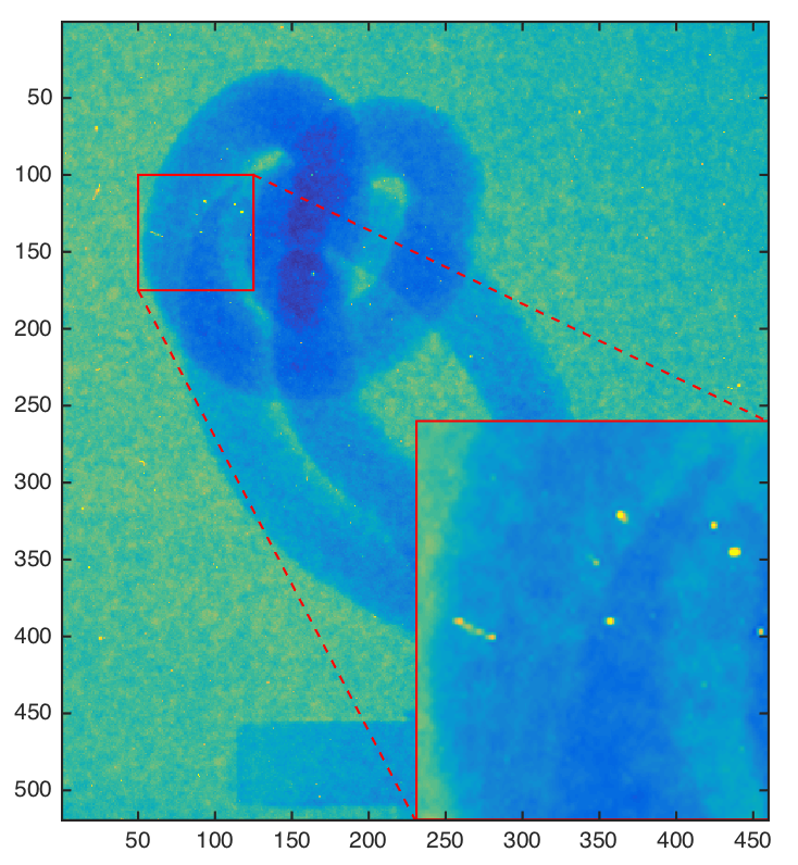
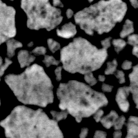
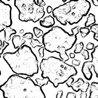
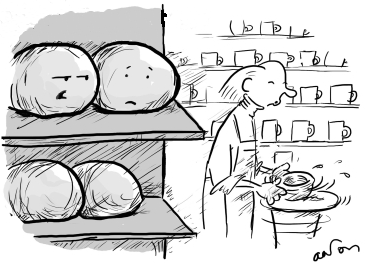
# ## Filter example: Spot cleaning
# 
# 
# 
# <table>
# <tr><th width="45%">Problem</th><th width="20%">Example</th><th width="35%">Possible solutions</th></tr>
# <tr><td>
#         
# - Many neutron images are corrupted by spots that confuse following processing steps. 
# - The amount, size, and intensity varies with many factors.   
# 
# </td>
# <td>
# <figure><img src="ext-figures/lecture03/spotty_knot_closeup.png" style="height:300px" align="middle"></figure>   
# </td>
# <td>
#     
# - Low pass filter
# - Median filter
# - Detect spots and replace by estimate
# 
# </td></tr>
# </table>

# ## Spot cleaning algorithm
# 
# <figure><img src="ext-figures/lecture03/spotclean_algorithm.svg" style="height:400px" align="middle"></figure>
# 
# #### Parameters
# 
# - $N$ Width of median filter.
# - $k$ Threshold level for outlier detection.
# 

# ## Spot cleaning - Compare performance
# <figure><img src="ext-figures/lecture03/spotclean_compare.svg"  style="height:500px" align="middle"></figure>
# 
# ### The ImageJ ways
# 
# - __Despeckle__ Median ... please avoid this one!!!
# - __Remove outliers__ Similar to cleaning described algorithm

# ## High-pass filters
# High-pass filters enhance rapid changes $\rightarrow$ ideal for edge detection
# 
# ### Typical high-pass filters:
# 
# #### Gradients
# $$\frac{\partial}{\partial\,x}=\frac{1}{2}\cdot\begin{array}{|c|c|}
# \hline
# -1 & 1\\
# \hline
# \end{array}\qquad
# \frac{\partial}{\partial\,x}=\frac{1}{32}\cdot\begin{array}{|c|c|c|}
# \hline
# -3 & 0 & 3\\
# \hline
# -10 & 0 & 10\\
# \hline
# -3 & 0 & 3\\
# \hline
# \end{array}
# $$
# #### Laplacian
# $$
# \bigtriangleup=\frac{1}{2}\cdot\begin{array}{|c|c|c|}
# \hline
# 1 & 2 & 1\\
# \hline
# 2 & -12 & 2\\
# \hline
# 1 & 2 & 1\\
# \hline
# \end{array}
# $$
# #### Sobel
# $$
# G=|\nabla f|=\sqrt{\left(\frac{\partial}{\partial\,x}f\right)^2 + \left(\frac{\partial}{\partial\,y}f\right)^2}
# $$
# 

# ## Gradient example

# #### Vertical edges
# $\frac{\partial}{\partial x}=\frac{1}{32}\cdot\begin{array}{|c|c|c|}
# \hline
# -3 & 0 & 3\\
# \hline
# -10 & 0 & 10\\
# \hline
# -3 & 0 & 3\\
# \hline
# \end{array}$  

# #### Horizontal egdges
# $\frac{\partial}{\partial\,y}=\frac{1}{32}\cdot\begin{array}{|c|c|c|}
# \hline
# -3 & -10 & -3\\
# \hline
# 0 & 0 & 0\\
# \hline
# 3 & 10 & 3\\
# \hline
# \end{array}$
# 
# [Jaehne, 2005](https://doi.org/10.1007/3-540-27563-0)

# In[ ]:


img=plt.imread('ext-figures/lecture03/orig.png')
k = np.array([[-3,-10,-3],[0,0,0],[3,10,3]]);
plt.figure(figsize=[15,8])
plt.subplot(1,3,1); plt.imshow(img);plt.title('Original');
plt.subplot(1,3,2); plt.imshow(ndimage.convolve(img,np.transpose(k)));plt.title('$\partial / \partial x$');
plt.subplot(1,3,3); plt.imshow(ndimage.convolve(img,k));plt.title('$\partial / \partial y$');


# ## Edge detection examples

# In[ ]:


img=plt.imread('ext-figures/lecture03/orig.png');
plt.figure(figsize=[15,6])
plt.subplot(1,2,1);plt.imshow(ski.filters.laplace(img),clim=[-0.08,0.08]); plt.title('Laplacian'); plt.colorbar();
plt.subplot(1,2,2);plt.imshow(ski.filters.sobel(img)); plt.title('Sobel');  plt.colorbar();


# ## Relevance of filters to machine learning
# <center><img src="ext-figures/lecture03/convolutional_neural_network.png"  style="height:500px" align="middle"></center>
# 	
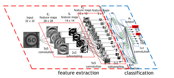
# [NVIDIA Developer zone](https://developer.nvidia.com/discover/convolutional-neural-network)
# 

# # Frequency space filters
# ## Applications of the Fourier transform

# ## The Fourier transform
# #### Transform
# $$G(\xi_1,\xi_2)=\mathcal{F}\{g\}=\int_{-\infty}^{\infty}\int_{-\infty}^{\infty} g(x,y)
# \exp{-i(\xi_1\,x+\xi_2\,y)}\,dx\,dy$$
# #### Inverse
# $$ g(x,y)=\mathcal{F}^{-1}\{G\}=\frac{1}{(2\,\pi)^2}\int_{-\infty}^{\infty}\int_{-\infty}^{\infty} G(\omega)
# \exp{i(\xi_1\,x+\xi_2\,y)}\,d\xi_1 \,d\xi_2$$
# 
# ### FFT (Fast Fourier Transform)
# In practice - you never see the transform equations. 
# The Fast Fourier Transform algorithm is available in numerical libraries and tools.
# 
# [Jaehne, 2005](https://doi.org/10.1007/3-540-27563-0)

# ## Some mathematical features of the FT
# #### Additition
# $\mathcal{F}\{a+b\} = \mathcal{F}\{a\}+\mathcal{F}\{b\}$

# In[ ]:


x = np.linspace(0,50,100); s0=np.sin(0.5*x); s1=np.sin(2*x);
plt.figure(figsize=[15,5])
plt.subplot(2,3,1);plt.plot(x,s0); plt.axis('off');plt.title('$s_0$');plt.subplot(2,3,4);plt.plot(np.abs(np.fft.fftshift(np.fft.fft(s0))));plt.axis('off');
plt.subplot(2,3,2);plt.plot(x,s1); plt.axis('off');plt.title('$s_1$');plt.subplot(2,3,5);plt.plot(np.abs(np.fft.fftshift(np.fft.fft(s1))));plt.axis('off');
plt.subplot(2,3,3);plt.plot(x,s0+s1); plt.axis('off');plt.title('$s_0+s_1$');plt.subplot(2,3,6);plt.plot(np.abs(np.fft.fftshift(np.fft.fft(s0+s1))));plt.axis('off');


# #### Convolution
# $\mathcal{F}\{a * b\} = \mathcal{F}\{a\} \cdot \mathcal{F}\{b\} $
# $\mathcal{F}\{a \cdot b\} = \mathcal{F}\{a\} * \mathcal{F}\{b\} $

# ## Additive noise in Fourier space
# #### Real space

# In[ ]:


img=plt.imread('ext-figures/lecture03/bp_ex_original.png'); noise=np.random.normal(0,0.2,size=img.shape); nimg=img+noise;
plt.figure(figsize=[15,3])
plt.subplot(1,3,1); plt.imshow(img);plt.title('Image');
plt.subplot(1,3,2); plt.imshow(noise);plt.title('Noise');
plt.subplot(1,3,3); plt.imshow(nimg);plt.title('Image + noise');


# #### Fourier space

# In[ ]:


plt.figure(figsize=[15,3])
plt.subplot(1,3,1); plt.imshow(np.log(np.abs(np.fft.fftshift(np.fft.fft2(img)))));plt.title('Image');
plt.subplot(1,3,2); plt.imshow(np.log(np.abs(np.fft.fftshift(np.fft.fft2(noise)))));plt.title('Noise');
plt.subplot(1,3,3); plt.imshow(np.log(np.abs(np.fft.fftshift(np.fft.fft2(nimg)))));plt.title('Image + noise');


# ### Problem
# How can we suppress noise without destroying relevant image features?

# ## Spatial frequencies and orientation

# In[ ]:


def ripple(size=128,angle=0,w0=0.1) :
    w=w0*np.linspace(0,1,size);
    [x,y]=np.meshgrid(w,w);
    img=np.sin((np.sin(angle)*x)+(np.cos(angle)*y));
    return img
N=64;
d0=ripple(N,angle=1/180*np.pi,w0=100);
d30=ripple(N,angle=30/180*np.pi,w0=100);
d60=ripple(N,angle=60/180*np.pi,w0=100);
d90=ripple(N,angle=89/180*np.pi,w0=100);
plt.figure(figsize=[15,8])
plt.subplot(2,4,1); plt.imshow(d0); plt.title('$0^{\circ}$'); plt.axis('off');
plt.subplot(2,4,2); plt.imshow(d30); plt.title('$30^{\circ}$'); plt.axis('off');
plt.subplot(2,4,3); plt.imshow(d60); plt.title('$60^{\circ}$'); plt.axis('off');
plt.subplot(2,4,4); plt.imshow(d90); plt.title('$90^{\circ}$'); plt.axis('off');

plt.subplot(2,4,5); plt.imshow((np.abs(np.fft.fftshift(np.fft.fft2(d0)))));   plt.axis('off');
plt.subplot(2,4,6); plt.imshow((np.abs(np.fft.fftshift(np.fft.fft2(d30)))));  plt.axis('off');
plt.subplot(2,4,7); plt.imshow((np.abs(np.fft.fftshift(np.fft.fft2(d60)))));  plt.axis('off');
plt.subplot(2,4,8); plt.imshow((np.abs(np.fft.fftshift(np.fft.fft2(d90)))));  plt.axis('off');


# ## Example - Stripe removal in Fourier space

# - Transform the image to Fourier space
# $$\mathcal{F_{2D}}\left\{a\right\} \Rightarrow A$$
# 
# - Multiply spectrum image by band pass filter
# $$A_{filtered}=A \cdot H$$
# 
# - Compute the inverse transform to obtain the filtered image in real space
# $$\mathcal{{F_{2D}}^{-1}}\left\{A_{filtered}\right\} \Rightarrow a_{filtered}$$

# In[ ]:


plt.figure(figsize=[8,10])
plt.subplot(4,1,1);plt.imshow(plt.imread('ext-figures/lecture03/raw_img.png')); plt.title('$a$'); plt.axis('off');
plt.subplot(4,1,2);plt.imshow(plt.imread('ext-figures/lecture03/raw_spec.png')); plt.title('$\mathcal{F}(a)$'); plt.axis('off');
plt.subplot(4,1,3);plt.imshow(plt.imread('ext-figures/lecture03/filt_spec.png')); plt.title('Kernel $H$'); plt.axis('off');
plt.subplot(4,1,4);plt.imshow(plt.imread('ext-figures/lecture03/filt_img.png')); plt.title('$a_{filtered}$'); plt.axis('off');


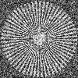
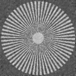
# ## The effect of the stripe filter
# 
# <table><tr><td> Reconstructed CT slice before filter</td><td>Reconstructed CT slice after stripe filter</td></tr>
#     <tr>
#         <td><img src="ext-figures/lecture03/slice_with_stripes.png"  style="height:400px" align="middle"></td>
#         <td><img src="ext-figures/lecture03/slice_stripe_filtered.png"  style="height:400px" align="middle"></td>
#     <tr></table>

# Intensity variations are suppressed using the stripe filter on all projections.

# ## Technical details on Fourier space filters
# #### When should you use convolution in Fourier space?
# -  Simplicity
# -  Kernel size
# -  Speed at repeated convolutions
# 
# #### Zero padding
# The FFT is only working with data of size in $2^N$. If your data has a different length, you have to pad (fill with constant value) up the next $2^N$.

# ## Python functions
# 	
# #### Filters in the spatial domain
# e.g. from ```scipy import ndimage```
# - ```ndimage.filters.convolve(f,h)``` Linear filter using kernel $h$ on image $f$.
# - ```ndimage.filters.median_filter(f,\[n,m\])```  Median filter using an $n \times m$ filter neighborhood
# 
# #### Fourier transform
# - ```np.fft.fft2(f)``` Computes the 2D Fast Fourier Transform of image $f$
# - ```np.fft.ifft2(F)``` Computes the inverse Fast Fourier Transform $F$.
# - ```np.fft.fftshift()``` Rearranges the data to center the $\omega$=0. Works for 1D and 2D.
# 
# #### Complex numbers
# - ```np.abs(f), np.angle(f)``` Computes amplitude and argument of a complex number.
# - ```np.real(f), np.imag(f)``` Gives the real and imaginary parts of a complex number.

# # Scale spaces

# ## Why scale spaces?

# ### Motivation
# Basic filters have problems to handle low SNR and textured noise.
# 
# Something new is required...
# ### The solution
# Filtering on different scales can take noise suppression one step further.

# <center><img src="ext-figures/lecture03/image_pyramid.svg"  style="height:400px" align="middle"></center>
# <font size="1">By <a href="//commons.wikimedia.org/wiki/User:Cmglee" title="User:Cmglee">Cmglee</a> - <span class="int-own-work" lang="en">Own work</span>, <a href="https://creativecommons.org/licenses/by-sa/3.0" title="Creative Commons Attribution-Share Alike 3.0">CC BY-SA 3.0</a>, <a href="https://commons.wikimedia.org/w/index.php?curid=42549151">Link</a></font>

# ## Wavelets - the basic idea
# - The wavelet transform produces scales by decomposing a signal into two signals at a coarser scale containing \emph{trend} and \emph{details}.\\
# - The next scale is computed using the trend of the previous transform
# $$WT\{s\}\rightarrow\{a_1,d_1\}, WT\{a_1\}\rightarrow\{a_2,d_2\}, \ldots, WT\{a_{N-1}\}\rightarrow\{a_N,d_N\} $$
# - The inverse transform brings $s$ back using $\{a_N,d_1, \ldots,d_N\}$.
# - Many wavelet bases exists, the choice depends on the application.
# 
# #### Applications of wavelets  
# - Noise reduction 
# - Analysis 
# - Segmentation
# - Compression
#     
# [Walker 2008](https://doi.org/10.1201/9781584887461) [Mallat 2009](https://doi.org/10.1016/B978-0-12-374370-1.X0001-8)

# ## Wavelet transform of a 1D signal
# 
# <center><img src="ext-figures/lecture03/wavelet1d_noaxis.svg" style="height:400px"></center>
# 
# Using __symlet-4__

# ## Wavelet transform of an image
# <center><img src="ext-figures/lecture03/wt2d_schematic.svg" style="height:400px"></center>

# ## Wavelet transform of an image - example
# 
# <table><tr><th>Original</th><th>Wavelet transformed</th></tr>
# <tr>
#     <td><img src="ext-figures/lecture03/testpattern_1024.png" style="height:400px"></td>
#     <td><img src="ext-figures/lecture03/wt_testimage_gray.png" style="height:400px"></td>
#     </tr>
#     </table>

# ## Wavelet noise reduction
# The noise is found in the detail part of the WT
# -  Make a WT of the signal to a level that corresponds to the scale of the unwanted information.
# - Threshold the detail part $d_{\gamma}=|d|<\gamma \,?\, 0 : d$.
# - Inverse WT back to normal scale $\rightarrow$ image is filtered.
# 
# <center><img src="ext-figures/lecture03/wavelet1d_filter.svg" style="height:400px"></center>

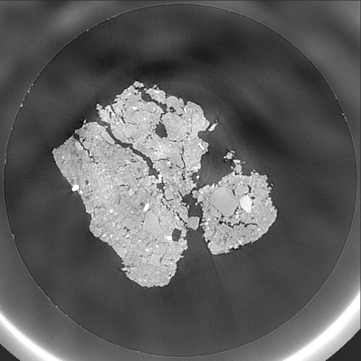
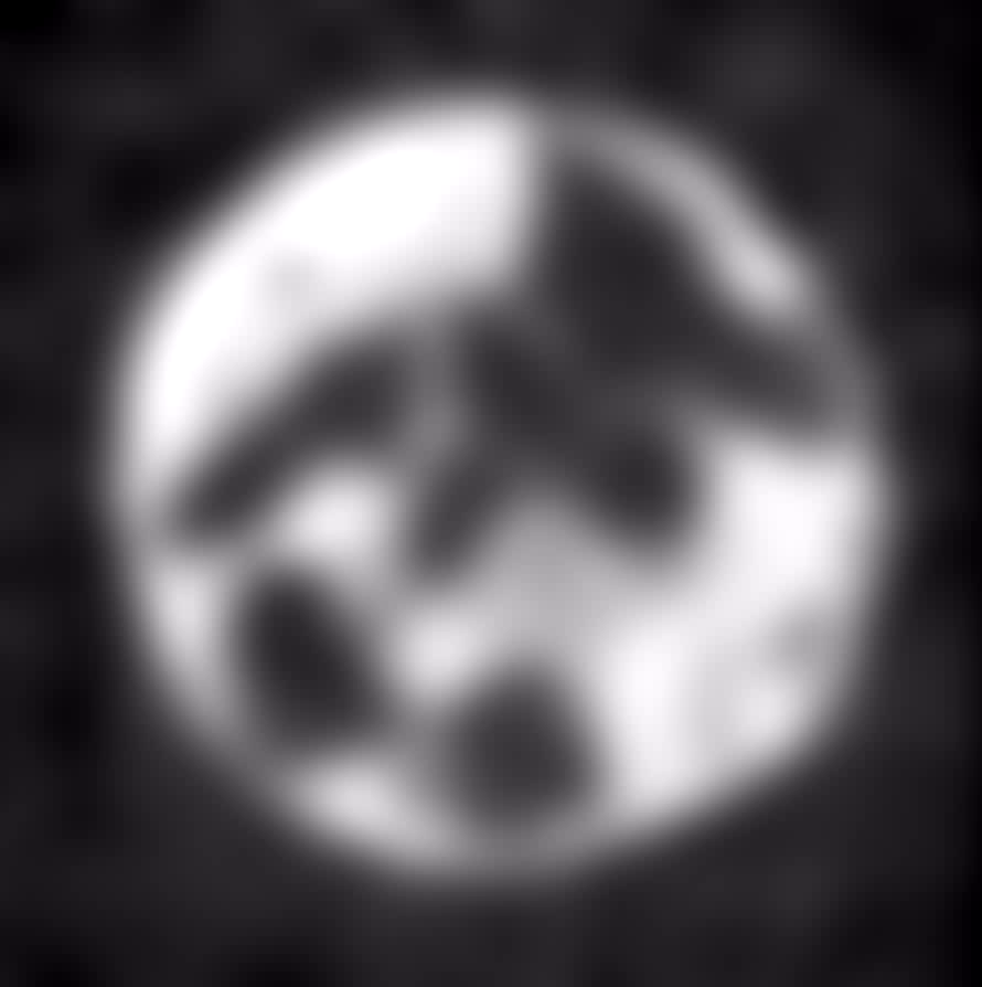
# ## Wavelet noise reduction - Image example
# #### Example Filtered using two levels of Symlet-2 wavelet
# __Data:__ Neutron CT of a lead scroll
# <center><img src="ext-figures/lecture03/wavelet2d_filtered.svg" style="height:400px"></center>

# ## Python functions
# ### dwt2/idtw2
# Makes one level of the wavelet transform or its inverse using wavelet base specified by 'wn'. 
# 
# ### wavedec2
# Performs N levels of wavelet decomposition using a specified wavelet base.
# ### wbmpen
# Estimating threshold parameters for wavelet denoising.
# ### wdencmp
# Wavelet denoising and compression using information from *wavedec2* and *wbmpen.
# 

# # Parameterized scale spaces
# 
# ## PDE based scale space filters
# <table><tr>
#     <td><img src="ext-figures/lecture03/slice_original.svg"  style="height:300px"></td>
#     <td><img src="ext-figures/lecture03/slice_diffusion.svg" style="height:300px"></td>
#     <td><img src="ext-figures/lecture03/slice_iss.svg"       style="height:300px"></td>
# </tr></table>
# 
# These filters may work for applications where Linear and Rank filters fail.
# 
# [Aubert 2002](https://doi.org/10.1007/978-0-387-44588-5).

# ## The starting point
# The heat transport equation
# $$\frac{\partial T}{\partial t}=\kappa\,\nabla^2 T$$
# 
# - __$T$__ Image to filter (intensity $\equiv$ temperature)
# - __$\kappa$__ Thermal conduction capacity
# <table>
#     <tr><td>Original</td><td>Iterations</td></tr>
#     <tr>
#           <td><img src="ext-figures/lecture03/lindif_iter.png" style="height:200px"></td>
#           <td><video src="ext-figures/lecture03/lindif_iter.mp4" type="video/mp4" controls autoplay loop height="200px"></td>
#     </tr>
#     </table>
# 
# <div class="alert alert-block alert-warning">
# <center>The steady state solution is a homogeneous image...</center>
# </div>
# 
# 

# ## Controlling the diffusivity

# In[ ]:


def g(x,lambd,n) :
    g=1/(1+(x/lambd)**n)
    return g


# We want to control the diffusion process...
# 
# - _Near edges_ The Diffusivity $\rightarrow$ 0
# - _Flat regions_ The Diffusivity $\rightarrow$ 1
# 
# The contrast function $G$ is our control function
# $$G(x)=\frac{1}{1+\left(\frac{x}{\lambda}\right)^n}$$
# 
# - _$\lambda$_ Threshold level
# - _$n$_ Steepness of the threshold function

# In[ ]:


x=np.linspace(0,1,100);

plt.plot(x,g(x,lambd=0.5,n=12));
plt.xlabel('Image intensity (x)'); plt.ylabel('G(x)');plt.tight_layout()


# ## Gradient controlled diffusivity
# 
# <font size=4>
# $$\frac{\partial u}{\partial t}=G(|\nabla u|)\,\nabla^2 u$$
# </font>
# <table><tr>
#       <td><img src="ext-figures/lecture03/aggregates.png"  style="height:300px"></td>
#   <td><img src="ext-figures/lecture03/diffusivity.png"  style="height:300px"></td>
#     </tr>
#     <tr>
# <td>Image</td><td>Diffusivity map</td>
# </tr></table>
# 
# - _$u$_ Image to be filtered
# - _$G(\cdot)$_ Non-linear function to control the diffusivity
# - _$\tau$_ Time increment
# - _$N$_ Number of iterations
# <div class="alert alert-block alert-danger">
# <center>This filter is noise sensitive!</center>
# </div>
# 
# 

# ## The non-linear diffusion filter
# A more robust filter is obtained with
# <font size=4>
# $$\frac{\partial u}{\partial t}=G(|\nabla_{\sigma} u|)\,\nabla^2 u$$
# </font>
# - _$u$_ Image to be filtered
# - _$G(\cdot)$_ Non-linear function to control the contrast
# - _$\tau$_ Time increment per numerical iteration
# - _$N$_ Number of iterations
# - _$\nabla_{\sigma}$_ Gradient smoothed by a Gaussian filter, width $\sigma$
# 
# 

# ## Diffusion filter example
# Neutron CT slice from a real-time experiment observing the coalescence of cold mixed bitumen.
# 
# <table>    
#     <tr>
#         <td>Original</td><td>Iterations of non-linear diffusion</td>
#     </tr>
#     <tr>
#         <td><img src="ext-figures/lecture03/bitumen.png" style="height:300px"></td>
#         <td><video src="ext-figures/lecture03/nldif_iter.mp4" type="video/mp4" controls autoplay loop height="300px"></td>    
#     </tr>
# </table>
# 

# ## Filtering as a regularization problem
# ### The continued development
# 
# - __90's__ During the late 90's the diffusion filter was described in terms of a regularization problem.
# - __00's__ Work toward regularization of total variation minimization.
# 
# #### TV-L1
# $$u=\underset{u\in BV(\Omega)}{\operatorname{argmin}}\left\{\underbrace{|u|_{BV}}_{noise}+ \underbrace{\mbox{$\frac{\lambda}{2}$}\|f-u\|_{1}}_{fidelity}\right\}$$
# #### Rudin-Osher-Fatemi model (ROF)
# $$u=\underset{u\in BV(\Omega)}{\operatorname{argmin}}\left\{\underbrace{|u|_{BV}}_{noise}+ \underbrace{\mbox{$\frac{\lambda}{2}$}\|f-u\|^2_{2}}_{fidelity}\right\}$$
# 
# with $|u|_{BV}=\int_{\Omega}|\nabla u|^2$
# 

# ## The inverse scale space filter
# #### The idea 
# We want smooth regions with sharp edges\ldots
# 
# - Turn the processing order of scale space filter upside down
# - Start with an empty image
# -  Add large structures successively until an image with relevant features appears
# 
# #### The ISS filter - Some properties
# - is an edge preserving filter for noise reduction.
# - is defined by a partial differential equation.
# - has a well defined termination point.
# 
# [Burger et al. 2006](https://dx.doi.org/10.4310/CMS.2006.v4.n1.a7)

# ## The ROF filter equation
# The image $f$ is filtered by solving
# 
# $$\begin{eqnarray}
# \frac{\partial u}{\partial t}&=& \mathrm{div}\left(\frac{\nabla u}{|\nabla u|}\right)+\lambda\,(f-u+v)\nonumber\\
# \frac{\partial v}{\partial t}&=& \alpha\, (f-u)
# \end{eqnarray}$$
# 
# #### Variables:
# - _$f$_ Input image
# - _$u$_ Filtered image
# - _$v$_ Regularization term (feedback of previous iteration)
# 
# #### Filter parameters
# - _$\lambda$_ Related to the scale of the features to suppress.
# - _$\alpha$_ Quality refinement
# - _$N$_ Number of iterations
# - _$\tau$_ Time increment
# 

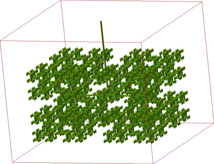
# ## Filter iterations
# Neutron CT of dried lung filtered using 3D ISS filter
# 
# <table>    
#     <tr><td>Original</td><td>Filter iterations</td></tr>
#     <tr>
#     <td><img src="ext-figures/lecture03/lung_iterations_first.png" style="height:300px"></td>   
#     <td><video src="ext-figures/lecture03/filter_iterations.mp4" type="video/mp4" controls autoplay loop height="300px"></td>
#     </tr>
# </table>
# 

# ## How to choose $\lambda$ and $\alpha$
# The requirements varies between different data sets.
# 
# #### Initial conditions:
# - Signal to noise ratio
# - Image features (fine grained or wide spread)
# 
# #### Experiment:
# - Scan $\lambda$ and $\alpha$
# - Stop at $T=n\, \tau= \sigma$ use different $\tau$
# - When does different effects occur, related to $\sigma$?

# ## Solutions at different times
# <table><tr><td>1</td><td>30</td><td>60</td><td>100</td><td>200</td><td>500</td><td>999</td></tr>
#     <tr>
#         <td><img src="ext-figures/lecture03/iss-iteration_0001.png" style="height:150px"></td>
#         <td><img src="ext-figures/lecture03/iss-iteration_0030.png" style="height:150px"></td>
#         <td><img src="ext-figures/lecture03/iss-iteration_0060.png" style="height:150px"></td>
#         <td><img src="ext-figures/lecture03/iss-iteration_0100.png" style="height:150px"></td>
#         <td><img src="ext-figures/lecture03/iss-iteration_0200.png" style="height:150px"></td>
#         <td><img src="ext-figures/lecture03/iss-iteration_0500.png" style="height:150px"></td>
#         <td><img src="ext-figures/lecture03/iss-iteration_0999.png" style="height:150px"></td>
#     </tr>
# </table>
# <img src="ext-figures/lecture03/iss-errorplot.svg" style="height:400px">
# 
# 
# 
# 

# ## Solution time
# The solution time ($T=N\cdot\tau$) is essential to the result
# - _$\tau$ large_ The solution is reached fast
# - _$\tau$ small_ The numerical accuracy is better

# ## The choice of initial image
# <img src="ext-figures/lecture03/iss-errorplots_initialimage.svg" style="height:400px">
# 
# At some $T$ the solution with $u_0=f$ and $u_0=0$ converge.

# # Non-local means

# ## Non-local smoothing
# ### The idea
# Smoothing normally consider information from the neighborhood like
# 
# - Local averages (convolution)
# - Gradients and Curvatures (PDE filters)
# 
# Non-local smoothing average similiar intensities in a global sense.
# - Every filtered pixel is a weighted average of all pixels.
# - Weights computed using difference between pixel intensities.
# 
# [Buades et al. 2005](http://dx.doi.org/10.1137/040616024)
# 

# ## Filter definition
# The non-local means filter is defined as
# $$u(p)=\frac{1}{C(p)}\sum_{q\in\Omega}v(q)\,f(p,q)$$
# where
# - _$v$ and $u$_ input and result images.
# - _$C(p)$_ is the sum of all pixel weights as 
# 
#     $C(p)=\sum_{q\in\Omega}f(p,q)$
#     
#     
# - _$f(p,q)$_ is the weighting function
# 
#     $f(p,q)=e^{-\frac{|B(q)-B(p)|^2}{h^2}}$
#     
#     
# - _B(x)_ is a neighborhood operator e.g. local average around $x$

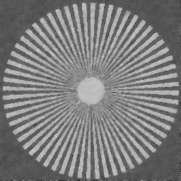
# ## Non-local means 2D - Example
# 
# <img src="ext-figures/lecture03/nonlocal_example.png" style="height:400px">
# 
# #### Observations
# 
# - Good smoothing effect.
# - Strong thin lines are preserved.
# -  Some patchiness related to filter parameter $t$, *i.e.* the size of $\Omega_i$.
# 

# ## Performance complications
# ### Problem
# The orignal filter compares all pixels with all pixels\ldots\\
# - Complexity $\mathcal{O}(N^2)$ 
# - Not feasible for large images, and particular 3D images!
# 
# ### Solution
# It has been shown that not all pixels have to be compared to achieve a good filter effect.
# i.e. $\Omega$ in the filter equations can be replaced by $\Omega_i<<\Omega$ 

# # Verification
# ## How good is my filter?

# ## Verify the correctness of the method
# #### "Data massage"
# Filtering manipulates the data, avoid too strong modifications otherwise you may invent new image features!!!
# 
# <center><img src="ext-figures/lecture03/mugs.png" style="height:250px"></center>
# 
# #### Verify the validity your method
# - Visual inspection
# - Difference images
# - Use degraded phantom images in a "smoke test"

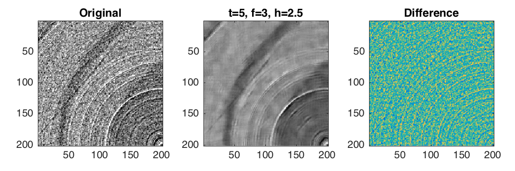
# ## Verification using difference images
# Compute pixel-wise difference between image $f$ and $g$
# <img src="ext-figures/lecture03/verification_differences.svg" style="height:600px">
# 
# Difference images provide first diagnosis about processing performance 

# ## Performance testing - The smoke test
# 
# - Testing term from electronic hardware testing - drive the system until something fails due to overheating...
# - In general: scan the parameter space for different SNR until the method fails to identify strength and weakness of the system.
# 
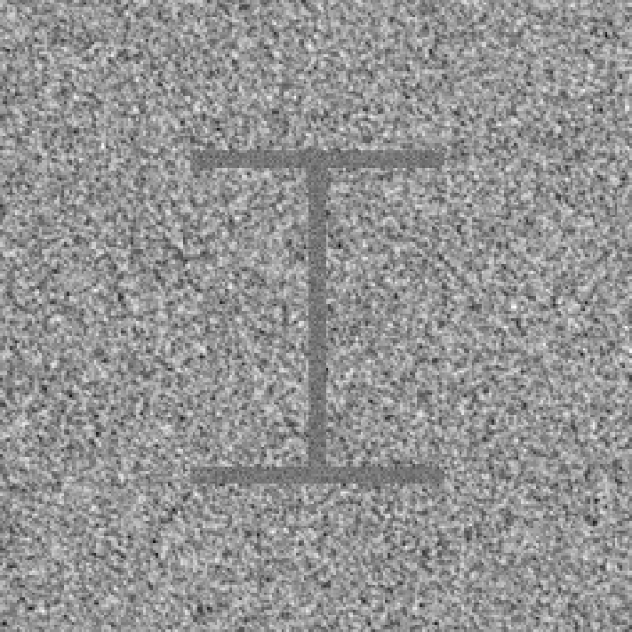
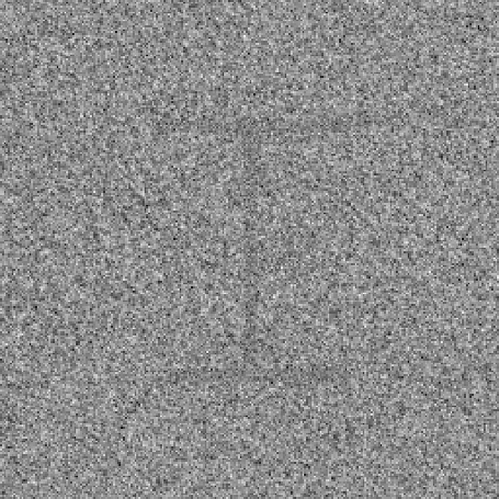
# ### Test strategy
# 1. Create a phantom image with relevant features.
# 2. Add noise for different SNR to the phantom.
# 3. Apply the processing method with different parameters.
# 4. Measure the difference between processed and phantom.
# 5. Repeat steps 2-4 $N$ times for better test statistics.
# 6. Plot the results and identify the range of SNR and parameters that produce acceptable results.

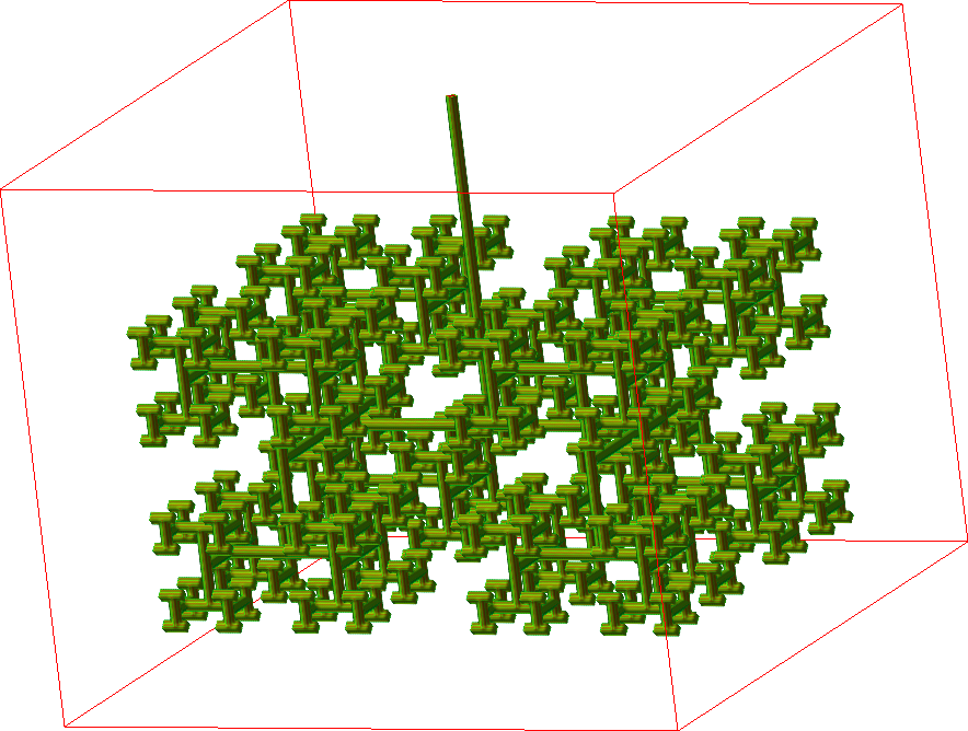
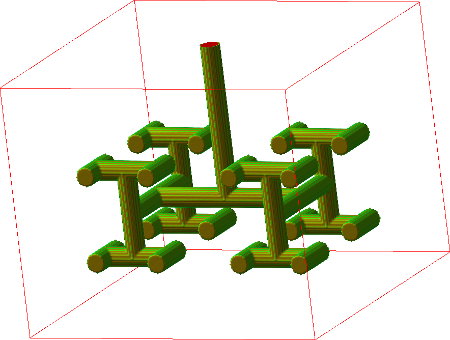
# ## Data for evaluation -  Phantom data
# General purpose can be controlled
# - Data with known features.
# - Parameters can be changed.
#     - Shape
#     - Sharpness
#     - Contrast
#     - Noise (distribution and strength)
# <table><tr>
# <td><img src="ext-figures/lecture03/shepplogan.png" style="height:250px"</td>
# <td><img src="ext-figures/lecture03/synthetic_root4.png" style="height:250px"</td>
#     </tr></table>

# ## Data for evaluation - Labelled data
# Often 'real' data
# - Labeled by experts
# - Used for training and validation
#      - Training of model
#      - Validation 
#      - Test
# 
# <center><img src="ext-figures/lecture03/mnist.png" style="height:300px"></center>

# ## Evaluation metrics for images
# An evaluation procedure need a metric to compare the performance
# #### Mean squared error
# <font size=5>
# $$MSE(f,g)=\sum_{p\in \Omega}(f(p)-g(p))^2$$
# </font>
# 
# #### Structural similarity index
# <font size=5>
# $$SSIM(f,g)=\frac{(2\mu_f\,\mu_g+C_1)(2\sigma_{fg}+C_2)}{(\mu_f^2+\mu_g^2+C_1)(\sigma_f^2+\sigma_g^2+C_2)}$$
#     </font>
#     
# - _$\mu_f$, $\mu_g$_ Local mean of $f$ and $g$.
# - _$\sigma_{fg}$_ Local correlation between $f$ and $g$.
# - _$\sigma_f$, $\sigma_g$_ Local standard deviation of $f$ and $g$.
# - _$C_1$, $C_2$_ Constants based on the image dynamics (small numbers).
# 
# 
# <font size=5>
# $$MSSIM(f,g)=E[SSIM(f,g)]$$
# </font>
# 
# [Wang 2009](https://doi.org/10.1109/MSP.2008.930649)

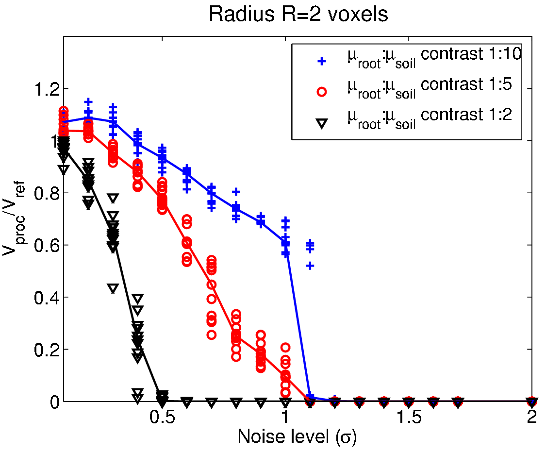
# ## Test run example
# #### Phantom structures
# <table><tr>
# <td><img src="ext-figures/lecture03/synthetic_root1.png" style="height:200px"></td>
# <td><img src="ext-figures/lecture03/synthetic_root2.png" style="height:200px"></td>
#     <td><img src="ext-figures/lecture03/synthetic_root4.png" style="height:200px"></td>
#     <td><img src="ext-figures/lecture03/synthetic_root8.png" style="height:200px"></td>
# </tr></table>
# 
# #### Change SNR and contrast
# <table><tr>
# <td><img src="ext-figures/lecture03/noise01.png" style="height:200px"></td>
# <td><img src="ext-figures/lecture03/noise02.png" style="height:200px"></td>
#     <td><img src="ext-figures/lecture03/noise05.png" style="height:200px"></td>
#     <td><img src="ext-figures/lecture03/noise10.png" style="height:200px"></td>
# </tr></table>

# #### Process
# 
# <div class="alert alert-block alert-success">
# Apply processing sequence.
# </div>
# 
# #### Plot results
# <table><tr>
# <td><img src="ext-figures/lecture03/radius1.png" style="height:200px"></td>
# <td><img src="ext-figures/lecture03/radius2.png" style="height:200px"></td>
#     <td><img src="ext-figures/lecture03/radius4.png" style="height:200px"></td>
#     <td><img src="ext-figures/lecture03/radius8.png" style="height:200px"></td>
# </tr></table>
# 
# [Kaestner et al. 2006](https://doi.org/10.1016/j.geoderma.2006.04.009)

# # Overview

# ## Many filters
# <img src="ext-figures/lecture03/filter_overview_gray.svg" style="height:600px">

# ## Details of filter performance
# 
# <img src="ext-figures/lecture03/filter_overview_close_gray.svg" style="height:600px">
# 

# ## Take-home message
# We have looked at different ways to suppress noise and artifacts:
# 
# - Convolution 
# - Median filters
# - Wavelet denoising
# - PDE filters
# 
# Which one you select depends on 
# - Purpose of the data
# - Quality requirements 
# - Available time
# <div class="alert alert-block alert-success">
# <b>Remember</b>: A good measurement is better than an enhanced bad measurement, but bad data can mostly be rescued if needed.
# </div>
# 
# 

# In[ ]: