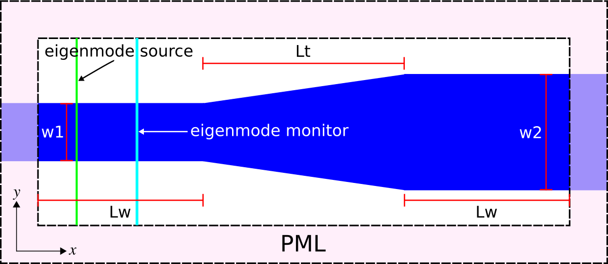
#!/usr/bin/env python # coding: utf-8 # ## Reflectance of a Waveguide Taper # # This example involves computing the reflectance of the fundamental mode of a linear waveguide taper. The structure and the simulation parameters are shown in the schematic below. We will verify that computing the reflectance, the fraction of the incident power which is reflected, using two different methods produces nearly identical results: (1) mode decomposition and (2) [Poynting flux](https://meep.readthedocs.io/en/latest/Introduction/#transmittancereflectance-spectra). Also, we will demonstrate that the scaling of the reflectance with the taper length is quadratic, consistent with analytical results from [Optics Express, Vol. 16, pp. 11376-92, 2008](http://www.opticsinfobase.org/abstract.cfm?URI=oe-16-15-11376). # # ![](https://meep.readthedocs.io/en/latest/images/waveguide-taper.png) # # The structure, which can be viewed as a [two-port network](https://en.wikipedia.org/wiki/Two-port_network), consists of a single-mode waveguide of width 1 μm (`w1`) at a wavelength of 6.67 μm and coupled to a second waveguide of width 2 μm (`w2`) via a linearly-sloped taper of variable length `Lt`. The material is silicon with ε=12. The taper geometry is defined using a single [`Prism`](https://meep.readthedocs.io/en/latest/Python_User_Interface/#prism) object with eight vertices. PML absorbing boundaries surround the entire cell. An eigenmode current source with E_z polarization is used to launch the fundamental mode. The dispersion relation (or "band diagram") of the single-mode waveguide is shown in [Tutorial/Eigenmode Source/Index-Guided Modes in a Ridge Waveguide](https://meep.readthedocs.io/en/latest/Python_Tutorials/Eigenmode_Source#index-guided-modes-in-a-ridge-waveguide). There is an eigenmode-expansion monitor placed at the midpoint of the first waveguide. This is a line monitor which extends beyond the waveguide in order to span the entire mode profile including its evanescent tails. The Fourier-transformed fields along this line monitor are used to compute the basis coefficients of the harmonic modes. These are computed separately via the eigenmode solver [MPB](https://mpb.readthedocs.io/en/latest/). This is described in [Mode Decomposition](https://meep.readthedocs.io/en/latest/Mode_Decomposition) where it is also shown that the squared magnitude of the mode coefficient is equivalent to the power (Poynting flux) in the given eigenmode. The ratio of the complex mode coefficients can be used to compute the [S parameters](https://en.wikipedia.org/wiki/Scattering_parameters). In this example, we are computing |S₁₁|² which is the reflectance (shown in the line prefixed by "refl:,"). Another line monitor could have been placed in the second waveguide to compute the transmittance or |S₂₁|² into the various guided modes (since the second waveguide is multi mode). The scattered power into the radiative modes can then be computed as 1-|S₁₁|²-|S₂₁|². Following usual practice, a normalization run is required involving a straight waveguide to compute the power in the source. # # The structure has mirror symmetry in the $y$ direction which can be exploited to reduce the computation size by a factor of two. This requires using `add_flux` rather than `add_mode_monitor` (which is not optimized for symmetry) and specifying the keyword argument `eig_parity=mp.ODD_Z+mp.EVEN_Y` in the call to `get_eigenmode_coefficients`. Alternatively, the waveguide could have been oriented along an arbitrary oblique direction which would require specifying `direction=mp.NO_DIRECTION` and `kpoint_func` as the waveguide axis. For an example, see [Tutorials/Eigenmode Source/Index-Guided Modes in a Ridge Waveguide](https://meep.readthedocs.io/en/latest/Python_Tutorials/Eigenmode_Source/#index-guided-modes-in-a-ridge-waveguide). # In[1]: import meep as mp import matplotlib.pyplot as plt resolution = 25 # pixels/μm w1 = 1.0 # width of waveguide 1 w2 = 2.0 # width of waveguide 2 Lw = 10.0 # length of waveguides 1 and 2 # lengths of waveguide taper Lts = [2**m for m in range(4)] dair = 3.0 # length of air region dpml_x = 6.0 # length of PML in x direction dpml_y = 2.0 # length of PML in y direction sy = dpml_y+dair+w2+dair+dpml_y Si = mp.Medium(epsilon=12.0) boundary_layers = [mp.PML(dpml_x,direction=mp.X), mp.PML(dpml_y,direction=mp.Y)] lcen = 6.67 # mode wavelength fcen = 1/lcen # mode frequency symmetries = [mp.Mirror(mp.Y)] R_coeffs = [] R_flux = [] for Lt in Lts: sx = dpml_x+Lw+Lt+Lw+dpml_x cell_size = mp.Vector3(sx,sy,0) src_pt = mp.Vector3(-0.5*sx+dpml_x+0.2*Lw) sources = [mp.EigenModeSource(src=mp.GaussianSource(fcen,fwidth=0.2*fcen), center=src_pt, size=mp.Vector3(y=sy-2*dpml_y), eig_match_freq=True, eig_parity=mp.ODD_Z+mp.EVEN_Y)] # straight waveguide vertices = [mp.Vector3(-0.5*sx-1,0.5*w1), mp.Vector3(0.5*sx+1,0.5*w1), mp.Vector3(0.5*sx+1,-0.5*w1), mp.Vector3(-0.5*sx-1,-0.5*w1)] sim = mp.Simulation(resolution=resolution, cell_size=cell_size, boundary_layers=boundary_layers, geometry=[mp.Prism(vertices,height=mp.inf,material=Si)], sources=sources, symmetries=symmetries) mon_pt = mp.Vector3(-0.5*sx+dpml_x+0.7*Lw) flux = sim.add_flux(fcen,0,1,mp.FluxRegion(center=mon_pt,size=mp.Vector3(y=sy-2*dpml_y))) sim.run(until_after_sources=mp.stop_when_fields_decayed(50,mp.Ez,mon_pt,1e-9)) res = sim.get_eigenmode_coefficients(flux,[1],eig_parity=mp.ODD_Z+mp.EVEN_Y) incident_coeffs = res.alpha incident_flux = mp.get_fluxes(flux) incident_flux_data = sim.get_flux_data(flux) sim.reset_meep() # linear taper vertices = [mp.Vector3(-0.5*sx-1,0.5*w1), mp.Vector3(-0.5*Lt,0.5*w1), mp.Vector3(0.5*Lt,0.5*w2), mp.Vector3(0.5*sx+1,0.5*w2), mp.Vector3(0.5*sx+1,-0.5*w2), mp.Vector3(0.5*Lt,-0.5*w2), mp.Vector3(-0.5*Lt,-0.5*w1), mp.Vector3(-0.5*sx-1,-0.5*w1)] sim = mp.Simulation(resolution=resolution, cell_size=cell_size, boundary_layers=boundary_layers, geometry=[mp.Prism(vertices,height=mp.inf,material=Si)], sources=sources, symmetries=symmetries) flux = sim.add_flux(fcen,0,1,mp.FluxRegion(center=mon_pt,size=mp.Vector3(y=sy-2*dpml_y))) sim.load_minus_flux_data(flux,incident_flux_data) sim.run(until_after_sources=mp.stop_when_fields_decayed(50,mp.Ez,mon_pt,1e-9)) res2 = sim.get_eigenmode_coefficients(flux,[1],eig_parity=mp.ODD_Z+mp.EVEN_Y) taper_coeffs = res2.alpha taper_flux = mp.get_fluxes(flux) R_coeffs.append(abs(taper_coeffs[0,0,1])**2/abs(incident_coeffs[0,0,0])**2) R_flux.append(-taper_flux[0]/incident_flux[0]) print("refl:, {}, {:.8f}, {:.8f}".format(Lt,R_coeffs[-1],R_flux[-1])) # Note that the reflectance is computed for five different geometrically-scaled taper lengths: 1, 2, 4, 8, and 16 μm. A quadratic scaling of the reflectance with the taper length appears as a straight line on a log-log plot. The results are plotted below. # In[2]: plt.figure(dpi=200) plt.loglog(Lts,R_coeffs,'bo-',label='mode decomposition') plt.loglog(Lts,R_flux,'ro-',label='Poynting flux') plt.loglog(Lts,[0.005/Lt**2 for Lt in Lts],'k-',label=r'quadratic reference (1/Lt$^2$)') plt.legend(loc='upper right') plt.xlabel('taper length Lt (μm)') plt.ylabel('reflectance') plt.show() # The reflectance values computed using the two methods are nearly identical. For reference, a line with quadratic scaling is shown in black. The reflectance of the linear waveguide taper decreases quadratically with the taper length which is consistent with the analytic theory. # # In the reflected-flux calculation, we apply our usual trick of first performing a reference simulation with just the incident field and then subtracting that from our taper simulation with `load_minus_flux_data`, so that what is left over is the reflected fields (from which we obtain the reflected flux). In *principle*, this trick would not be required for the mode-decomposition method, because the reflected mode is orthogonal to the forward mode and so the decomposition will separate the forward and reflected coefficients automatically. However, this is only true in the limit of infinite resolution — for a *finite* resolution, the reflected mode used for the mode coefficient calculation (calculated via MPB) is not exactly orthogonal to the forward mode propagating in Meep (whose discretization scheme is different from that of MPB). In consequence, if you did not subtract the fields of the reference simulation, the mode-coefficient could only calculate the reflected power down to a "noise floor" set by the discretization error. With the subtraction, in contrast, you can compute much smaller reflections (limited by the floating-point precision).