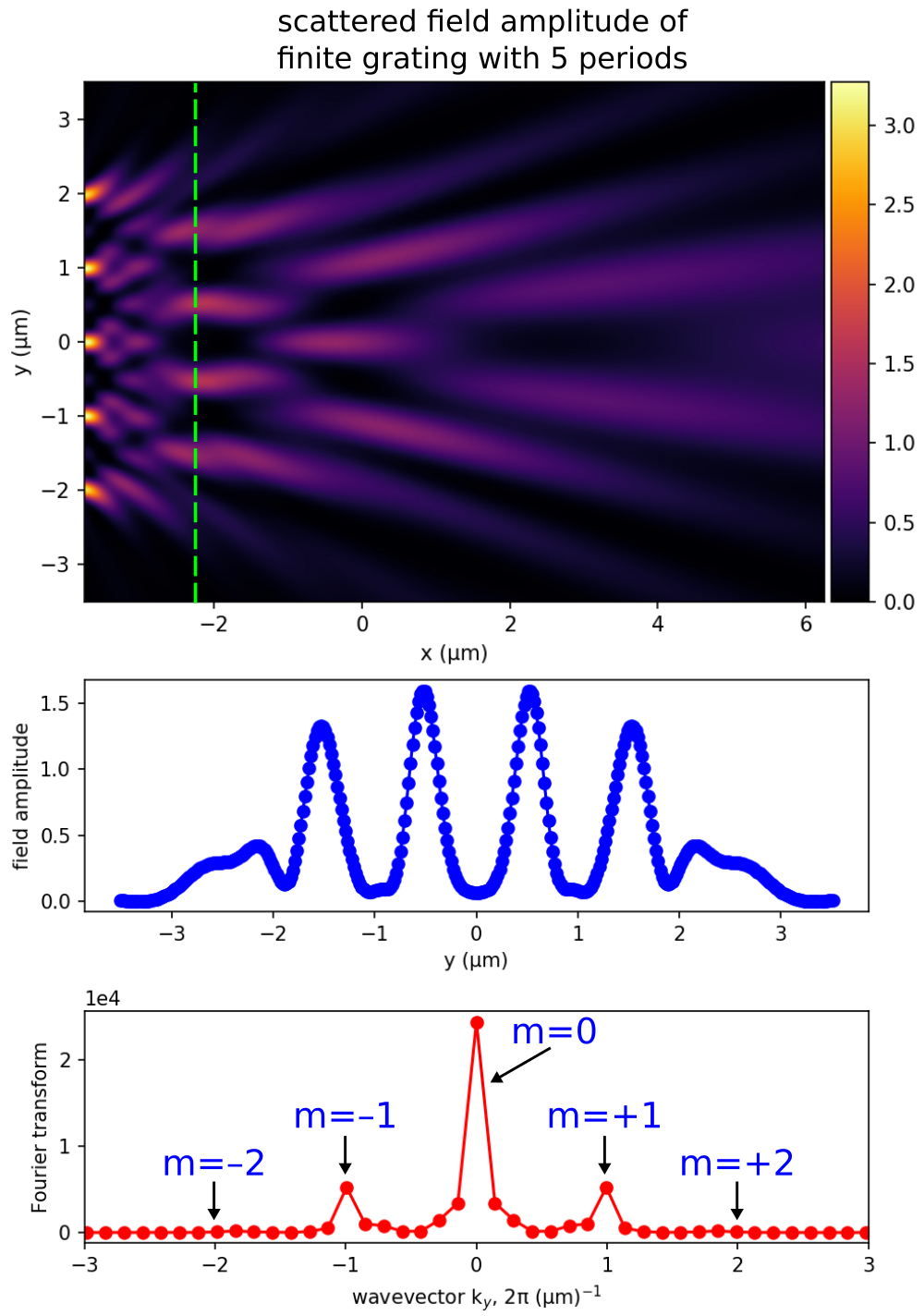
#!/usr/bin/env python # coding: utf-8 # # Diffraction Spectrum of a Finite Binary Grating # Finally, we can validate the results for the diffraction spectra of a finite grating via a different approach than computing the far fields: as the (spatial) Fourier transform of the scattered fields. This involves two simulations — one with the grating and the other with just a flat surface — and subtracting the Fourier-transformed fields at a given frequency ω from the two runs to obtain the scattered fields s(y). The Fourier transform of the scattered fields is then computed in post processing: a(k_y) = ∫ s(y) exp(ik_yy) dy, where |a(k_y)|² is the amplitude of the corresponding Fourier component. For a grating with periodicity Λ, we should expect to see peaks in the diffraction spectra at k_y=2πm/Λ for m=0, ±1, ±2, ... The total number of diffraction orders is determined by the wavelength as described in [Tutorials/Mode Decomposition/Transmittance Spectra for Planewave at Normal Incidence](https://meep.readthedocs.io/en/latest/Python_Tutorials/Mode_Decomposition/#transmittance-spectra-for-planewave-at-normal-incidence). 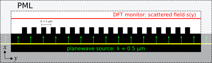# # The simulation setup is shown in the schematic below. The binary grating has Λ = 1 μm at a wavelength of 0.5 μm via a normally-incident planewave pulse (which must [extend into the PML region in order to span the entire width of the cell](https://meep.readthedocs.io/en/latest/Perfectly_Matched_Layer/#planewave-sources-extending-into-pml)). The grating structure is terminated with a flat-surface padding in order to give the scattered field space to decay at the edge of the cell. # # ![](https://meep.readthedocs.io/en/latest/images/finite_grating_schematic.png) # In[1]: import meep as mp import numpy as np import math import matplotlib.pyplot as plt # True: plot the scattered fields in the extended air region adjacent to the grating # False: plot the diffraction spectra based on a 1d cross section of the scattered fields field_profile = True resolution = 50 # pixels/μm dpml = 1.0 # PML thickness dsub = 2.0 # substrate thickness dpad = 1.0 # flat-surface padding gp = 1.0 # grating periodicity gh = 0.5 # grating height gdc = 0.5 # grating duty cycle num_cells = 5 # number of grating unit cells # air region thickness adjacent to grating dair = 10 if field_profile else dpad wvl = 0.5 # center wavelength fcen = 1/wvl # center frequency k_point = mp.Vector3() glass = mp.Medium(index=1.5) pml_layers = [mp.PML(thickness=dpml)] symmetries=[mp.Mirror(mp.Y)] sx = dpml+dsub+gh+dair+dpml sy = dpml+dpad+num_cells*gp+dpad+dpml cell_size = mp.Vector3(sx,sy) src_pt = mp.Vector3(-0.5*sx+dpml+0.5*dsub) sources = [mp.Source(mp.GaussianSource(fcen,fwidth=0.2*fcen), component=mp.Ez, center=src_pt, size=mp.Vector3(y=sy))] geometry = [mp.Block(material=glass, size=mp.Vector3(dpml+dsub,mp.inf,mp.inf), center=mp.Vector3(-0.5*sx+0.5*(dpml+dsub)))] sim = mp.Simulation(resolution=resolution, cell_size=cell_size, boundary_layers=pml_layers, geometry=geometry, k_point=k_point, sources=sources, symmetries=symmetries) mon_pt = mp.Vector3(0.5*sx-dpml-0.5*dair) near_fields = sim.add_dft_fields([mp.Ez], fcen, 0, 1, center=mon_pt, size=mp.Vector3(dair if field_profile else 0,sy-2*dpml)) sim.run(until_after_sources=100) flat_dft = sim.get_dft_array(near_fields, mp.Ez, 0) sim.reset_meep() for j in range(num_cells): geometry.append(mp.Block(material=glass, size=mp.Vector3(gh,gdc*gp,mp.inf), center=mp.Vector3(-0.5*sx+dpml+dsub+0.5*gh,-0.5*sy+dpml+dpad+(j+0.5)*gp))) sim = mp.Simulation(resolution=resolution, cell_size=cell_size, boundary_layers=pml_layers, geometry=geometry, k_point=k_point, sources=sources, symmetries=symmetries) near_fields = sim.add_dft_fields([mp.Ez], fcen, 0, 1, center=mon_pt, size=mp.Vector3(dair if field_profile else 0,sy-2*dpml)) sim.run(until_after_sources=100) # In[2]: grating_dft = sim.get_dft_array(near_fields, mp.Ez, 0) scattered_field = grating_dft-flat_dft scattered_amplitude = np.abs(scattered_field)**2 [x,y,z,w] = sim.get_array_metadata(dft_cell=near_fields) if field_profile: plt.figure(dpi=150) plt.pcolormesh(x,y,np.rot90(scattered_amplitude),cmap='inferno',shading='gouraud',vmin=0,vmax=scattered_amplitude.max()) plt.gca().set_aspect('equal') plt.xlabel('x (μm)') plt.ylabel('y (μm)') # ensure that the height of the colobar matches that of the plot from mpl_toolkits.axes_grid1 import make_axes_locatable divider = make_axes_locatable(plt.gca()) cax = divider.append_axes("right", size="5%", pad=0.05) plt.colorbar(cax=cax) plt.tight_layout() plt.show() else: ky = np.fft.fftshift(np.fft.fftfreq(len(scattered_field), 1/resolution)) FT_scattered_field = np.fft.fftshift(np.fft.fft(scattered_field)) plt.figure(dpi=150) plt.subplots_adjust(hspace=0.3) plt.subplot(2,1,1) plt.plot(y,scattered_amplitude,'bo-') plt.xlabel("y (μm)") plt.ylabel("field amplitude") plt.subplot(2,1,2) plt.plot(ky,np.abs(FT_scattered_field)**2,'ro-') plt.gca().ticklabel_format(axis='y',style='sci',scilimits=(0,0)) plt.xlabel(r'wavevector k$_y$, 2π (μm)$^{-1}$') plt.ylabel("Fourier transform") plt.gca().set_xlim([-3, 3]) plt.tight_layout(pad=1.0) plt.show() # Results are shown for two finite gratings with 5 and 20 periods. # # ![](https://meep.readthedocs.io/en/latest/images/finite_grating_nperiods5.png) # # ![](https://meep.readthedocs.io/en/latest/images/finite_grating_nperiods20.png) # # The scattered field amplitude profile (the top figure in each of the two sets of results) shows that the fields are nonzero above the grating (which is positioned at the left edge of the figure in the region indicated by the bright spots) and decay to zero away from the grating. The middle figure is the field amplitude along a 1d slice at a distance 1.5 μm above the grating (marked by the dotted green line in the top figure). Note the decaying fields at the edges due to the flat-surface termination. The bottom figure is the Fourier transform of the fields from the 1d slice. As expected, there are only three diffraction orders present at k_y=2πm/Λ for m=0, ±1, ±2. These peaks are becoming sharper as the number of grating periods increases. # # The sharpness of the peaks directly corresponds to how [collimated](https://en.wikipedia.org/wiki/Collimated_beam) the diffracted beams are, and in the limit of infinitely many periods the resulting delta-function peaks correspond to diffracted planewaves. (The squared amplitude of each peak is proportional to the power in the corresponding diffraction order.) One can also obtain the collimation of the beams more directly by using Meep's `near2far` feature to compute the far-field diffracted waves — this approach is more straightforward, but potentially much more expensive than looking at the Fourier transform of the near field, because one may need a large number of far-field points to resolve the full diffracted beams. In general, [there is a tradeoff in computational science](https://icerm.brown.edu/video_archive/?play=1626) between doing direct "numerical experiments" that are conceptually straightforward but often expensive, versus more indirect and tricky calculations that don't directly correspond to laboratory experiments but which can sometimes be vastly more efficient at extracting physical information. # # In 3d, the procedure is very similar, but a little more effort is required to disentangle the two polarizations relative to the plane of incidence [the (z,**k**) plane for each Fourier component **k**]. For propagation in the $z$ direction, you would Fourier transform both $E_x$ and $E_y$ of the scattered field as a function of **k** $= (k_x, k_y)$. For each **k**, you decompose the corresponding **E** $= (E_x, E_y)$ into the amplitude parallel to **k** [which gives the *p* polarization amplitude if you multiply by csc(θ), where cos(θ)=|**k**|/(nω/c), n is the refractive index of the ambient medium, and ω is the angular frequency] and perpendicular to **k** [which equals the *s* polarization amplitude]. Then square these amplitudes to get something proportional to power as above. (Note that this analysis is the same even if the incident wave is at an oblique angle, although the **k** locations of the diffraction peaks will change.)