#!/usr/bin/env python # coding: utf-8 #

ATAR: Automatic and Tunable Artifact Removal Algorithm

1 ATAR: Automatic and Tunable Artifact Removal Algorithm
2 Import EEG sample data
- 2.1 Filter with highpass
3 Applying ATAR Algorithm
4 Other settings
5 Doc

# # ATAR: Automatic and Tunable Artifact Removal Algorithm # **ATAR Algorithm - Automatic and Tunable Artifact Removal Algorithm for EEG Signal.** # # The algorithm is based on wavelet packet decomposion (WPD), the full description of algorithm can be found here [Automatic and Tunable Artifact Removal Algorithm for EEG](https://doi.org/10.1016/j.bspc.2019.101624) from the article [1]. Figure 1 shows the the block diagram and operating mode of filtering. # #

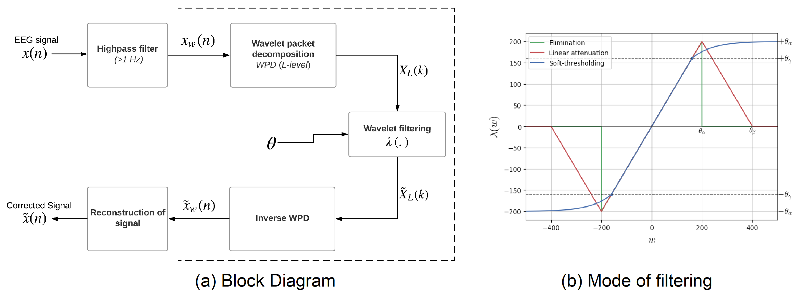
Fig 1: ATAR Algorithm Block Diagram and Mode of filtering

# # # The algorithm is applied on the given multichannel signal X (n,nch), window wise and reconstructed with overall add method. The defualt window size is set to 1 sec (128 samples). For each window, the threshold $\theta_\alpha$ is computed and applied to filter the wavelet coefficients. # # There is manily one parameter that can be tuned $\beta$ with different operating modes and other settings. # Here is the list of parameters and there simplified meaning given: # # Parameters: # * $\beta$: This is a main parameter to tune, highher the value, more aggressive the algorithm to remove the artifacts. By default it is set to 0.1. $\beta$ is postive float value. # # * ***OptMode***: This sets the mode of operation, which decides hoe to remove the artifact. By default it is set to 'soft', which means Soft Thresholding, in this mode, rather than removing the pressumed artifact, it is suppressed to the threshold, softly. OptMode='linAtten', suppresses the pressumed artifact depending on how far it is from threshold. Finally, the most common mode - Elimination (OptMode='elim'), which remove the pressumed artifact. # # * Soft Thresholding and Linear Attenuation require addition parameters to set the associated thresholds which are by default set to bf=2, gf=0.8. # # * ***wv=db3***: Wavelet funtion, by default set to db3, could be any of ['db3'.....'db38', 'sym2.....sym20', 'coif1.....coif17', 'bior1.1....bior6.8', 'rbio1.1...rbio6.8', 'dmey'] # # * $k_1$, $k_2$: Lower and upper bounds on threshold $\theta_\alpha$. # * ***IPR=[25,75]***: interpercentile range, range used to compute threshold # # Figure 2, below, shows the affect of $\beta$ on a segment of signal with three different modes. # #

Fig 1: ATAR Algorithm with three mode of filtering

# # # # **Reference** # * [1] Bajaj, Nikesh, et al. "Automatic and tunable algorithm for EEG artifact removal using wavelet decomposition with applications in predictive modeling during auditory tasks." Biomedical Signal Processing and Control 55 (2020): 101624. # There are three functions in **spkit.eeg** for **ATAR algorithm** # # * **spkit.eeg.ATAR(...)** # * spkit.eeg.ATAR_1Ch(...) # * spkit.eeg.ATAR_mCh(...) # * spkit.eeg.ATAR_mCh_noParallel(...) # # ***spkit.eeg.ATAR_1Ch*** is for single channel input signal x of shape (n,), where as, ***spkit.eeg.ATAR_mCh*** is for multichannel signal X with shape (n,ch), which uses joblib for parallel processing of multi channels. For some OS, joblib raise an error of ***BrokenProcessPool***, in that case use ***spkit.eeg.ATAR_mCh_noParallel***, which is same as ***spkit.eeg.ATAR_mCh***, except parallel processing. Alternatively, use ***spkit.eeg.ATAR_1Ch*** with for loop for each channel. # # ***spkit.eeg.ATAR*** is generalized function, this will call ***spkit.eeg.ATAR_1Ch*** is single channel is passed else ***spkit.eeg.ATAR_mCh*** and with *use_joblib* agrument, it can be set to try parallel processing, else will process each channel individually. We recommed to use ***spkit.eeg.ATAR***. # In[2]: import numpy as np import matplotlib.pyplot as plt import spkit as sp sp.__version__ # # Import EEG sample data # In[3]: X,ch_names = sp.load_data.eegSample() fs = 128 # In[4]: #help(sp.filter_X) # ## Filter with highpass # In[5]: Xf = sp.filter_X(X,band=[0.5], btype='highpass',fs=fs,verbose=0) Xf.shape # In[6]: t = np.arange(Xf.shape[0])/fs plt.figure(figsize=(12,5)) plt.plot(t,Xf+np.arange(-7,7)*200) plt.xlim([t[0],t[-1]]) plt.xlabel('time (sec)') plt.yticks(np.arange(-7,7)*200,ch_names) plt.grid() plt.title('Xf: 14 channel - EEG Signal (filtered)') plt.show() # # Applying ATAR Algorithm # ## Soft Thresholding: default settings: OptMode='soft' and $\beta=0.1$ # In[18]: XR = sp.eeg.ATAR(Xf.copy(),verbose=0) XR.shape # In[19]: plt.figure(figsize=(12,5)) plt.plot(t,XR+np.arange(-7,7)*200) plt.xlim([t[0],t[-1]]) plt.xlabel('time (sec)') plt.yticks(np.arange(-7,7)*200,ch_names) plt.grid() plt.title('XR: Corrected Signal') plt.show() plt.figure(figsize=(12,5)) plt.plot(t,(Xf-XR)+np.arange(-7,7)*200) plt.xlim([t[0],t[-1]]) plt.xlabel('time (sec)') plt.yticks(np.arange(-7,7)*200,ch_names) plt.grid() plt.title('Xf - XR: Difference (removed signal)') plt.show() # ## Linear Attenuation # In[20]: XR = sp.eeg.ATAR(Xf.copy(),verbose=0,OptMode='linAtten') XR.shape # In[21]: plt.figure(figsize=(12,5)) plt.plot(t,XR+np.arange(-7,7)*200) plt.xlim([t[0],t[-1]]) plt.xlabel('time (sec)') plt.yticks(np.arange(-7,7)*200,ch_names) plt.grid() plt.title('XR: Corrected Signal') plt.show() plt.figure(figsize=(12,5)) plt.plot(t,(Xf-XR)+np.arange(-7,7)*200) plt.xlim([t[0],t[-1]]) plt.xlabel('time (sec)') plt.yticks(np.arange(-7,7)*200,ch_names) plt.grid() plt.title('Xf - XR: Difference (removed signal)') plt.show() # ## Elimination # In[22]: XR = sp.eeg.ATAR(Xf.copy(),verbose=0,OptMode='elim') XR.shape # In[23]: plt.figure(figsize=(12,5)) plt.plot(t,XR+np.arange(-7,7)*200) plt.xlim([t[0],t[-1]]) plt.xlabel('time (sec)') plt.yticks(np.arange(-7,7)*200,ch_names) plt.grid() plt.title('XR: Corrected Signal') plt.show() plt.figure(figsize=(12,5)) plt.plot(t,(Xf-XR)+np.arange(-7,7)*200) plt.xlim([t[0],t[-1]]) plt.xlabel('time (sec)') plt.yticks(np.arange(-7,7)*200,ch_names) plt.grid() plt.title('Xf - XR: Difference (removed signal)') plt.show() # ## Tuning $\beta$ with 'soft' : Controlling the aggressiveness # In[24]: betas = np.r_[np.arange(0.01,0.1,0.02), np.arange(0.1,1, 0.1)].round(2) for b in betas: XR = sp.eeg.ATAR(Xf.copy(),verbose=0,beta=b,OptMode='soft') XR.shape plt.figure(figsize=(15,5)) plt.subplot(121) plt.plot(t,XR+np.arange(-7,7)*200) plt.xlim([t[0],t[-1]]) plt.xlabel('time (sec)') plt.yticks(np.arange(-7,7)*200,ch_names) plt.grid() plt.title('XR: Corrected Signal: '+r'$\beta=$' + f'{b}') plt.subplot(122) plt.plot(t,(Xf-XR)+np.arange(-7,7)*200) plt.xlim([t[0],t[-1]]) plt.xlabel('time (sec)') plt.yticks(np.arange(-7,7)*200,ch_names) plt.grid() plt.title('Xf - XR: Difference (removed signal)') plt.show() # ## Tuning $\beta$ with 'elim' # In[25]: betas = np.r_[np.arange(0.01,0.1,0.02), np.arange(0.1,1, 0.1)].round(2) for b in betas: XR = sp.eeg.ATAR(Xf.copy(),verbose=0,beta=b,OptMode='elim') XR.shape plt.figure(figsize=(15,5)) plt.subplot(121) plt.plot(t,XR+np.arange(-7,7)*200) plt.xlim([t[0],t[-1]]) plt.xlabel('time (sec)') plt.yticks(np.arange(-7,7)*200,ch_names) plt.grid() plt.title('XR: Corrected Signal: '+r'$\beta=$' + f'{b}') plt.subplot(122) plt.plot(t,(Xf-XR)+np.arange(-7,7)*200) plt.xlim([t[0],t[-1]]) plt.xlabel('time (sec)') plt.yticks(np.arange(-7,7)*200,ch_names) plt.grid() plt.title('Xf - XR: Difference (removed signal)') plt.show() # # Other settings # ## Changing wavelet function # In[26]: XR = sp.eeg.ATAR(Xf.copy(),wv='db8',beta=0.01,OptMode='elim',verbose=0,) XR.shape plt.figure(figsize=(15,5)) plt.subplot(121) plt.plot(t,XR+np.arange(-7,7)*200) plt.xlim([t[0],t[-1]]) plt.xlabel('time (sec)') plt.yticks(np.arange(-7,7)*200,ch_names) plt.grid() plt.title('XR: Corrected Signal: '+r'$wv=db8$') plt.subplot(122) plt.plot(t,(Xf-XR)+np.arange(-7,7)*200) plt.xlim([t[0],t[-1]]) plt.xlabel('time (sec)') plt.yticks(np.arange(-7,7)*200,ch_names) plt.grid() plt.title('Xf - XR: Difference (removed signal)') plt.show() XR = sp.eeg.ATAR_mCh_noParallel(Xf.copy(),wv='db32',beta=0.01,OptMode='elim',verbose=0,) XR.shape plt.figure(figsize=(15,5)) plt.subplot(121) plt.plot(t,XR+np.arange(-7,7)*200) plt.xlim([t[0],t[-1]]) plt.xlabel('time (sec)') plt.yticks(np.arange(-7,7)*200,ch_names) plt.grid() plt.title('XR: Corrected Signal: '+r'$wv=db32$') plt.subplot(122) plt.plot(t,(Xf-XR)+np.arange(-7,7)*200) plt.xlim([t[0],t[-1]]) plt.xlabel('time (sec)') plt.yticks(np.arange(-7,7)*200,ch_names) plt.grid() plt.title('Xf - XR: Difference (removed signal)') plt.show() # ## Changing upper and lower bounds: $k_1$, $k_2$ # $k_1$ and $k_2$ are lower and upper bound on the threshold $\theta_\alpha$. $k_1$ is set to 10, which means, the lowest threshold value will be 10, this helps to prevent the removal of entire signal (zeroing out) due to present of high magnitute of artifact. $k_2$ is largest threshold value, which in terms set the decaying curve of threshold $\theta_\alpha$. Increasing k2 will make the removal less aggressive # In[27]: XR = sp.eeg.ATAR(Xf.copy(),wv='db3',beta=0.1,OptMode='elim',verbose=0,k1=10, k2=200) XR.shape plt.figure(figsize=(15,5)) plt.subplot(121) plt.plot(t,XR+np.arange(-7,7)*200) plt.xlim([t[0],t[-1]]) plt.xlabel('time (sec)') plt.yticks(np.arange(-7,7)*200,ch_names) plt.grid() plt.title('XR: Corrected Signal: '+r'$k_2=200$') plt.subplot(122) plt.plot(t,(Xf-XR)+np.arange(-7,7)*200) plt.xlim([t[0],t[-1]]) plt.xlabel('time (sec)') plt.yticks(np.arange(-7,7)*200,ch_names) plt.grid() plt.title('Xf - XR: Difference (removed signal)') plt.show() # ## Changing IPR - Interpercentile range # **IPR is interpercentile range**, which is set to 50% (IPR=[25,75]) as default (inter-quartile range), incresing the range increses the aggressiveness of removing artifacts. # In[28]: XR = sp.eeg.ATAR(Xf.copy(),wv='db3',beta=0.1,OptMode='elim',verbose=0,k1=10, k2=200, IPR=[15,85]) plt.figure(figsize=(15,5)) plt.subplot(121) plt.plot(t,XR+np.arange(-7,7)*200) plt.xlim([t[0],t[-1]]) plt.xlabel('time (sec)') plt.yticks(np.arange(-7,7)*200,ch_names) plt.grid() plt.title('XR: Corrected Signal: '+r'$IPR=[15,85]$~ 70%') plt.subplot(122) plt.plot(t,(Xf-XR)+np.arange(-7,7)*200) plt.xlim([t[0],t[-1]]) plt.xlabel('time (sec)') plt.yticks(np.arange(-7,7)*200,ch_names) plt.grid() plt.title('Xf - XR: Difference (removed signal)') plt.show() # ## Using the fix threshold $\theta_\alpha=300$, to all the windows # In[29]: XR = sp.eeg.ATAR(Xf.copy(),wv='db3',thr_method=None,theta_a=300,OptMode='elim',verbose=0) plt.figure(figsize=(15,5)) plt.subplot(121) plt.plot(t,XR+np.arange(-7,7)*200) plt.xlim([t[0],t[-1]]) plt.xlabel('time (sec)') plt.yticks(np.arange(-7,7)*200,ch_names) plt.grid() plt.title('XR: Corrected Signal: '+r'$\theta_\alpha=300$') plt.subplot(122) plt.plot(t,(Xf-XR)+np.arange(-7,7)*200) plt.xlim([t[0],t[-1]]) plt.xlabel('time (sec)') plt.yticks(np.arange(-7,7)*200,ch_names) plt.grid() plt.title('Xf - XR: Difference (removed signal)') plt.show() # ## Changing window length (5 sec) # **winsize** is be default set to 128 (1 sec), assuming 128 sampling rate, which can be changed as needed. In following example it is changed to 5 sec. # In[31]: XR = sp.eeg.ATAR(Xf.copy(),winsize=128*5,beta=0.01,OptMode='elim',verbose=0,) plt.figure(figsize=(15,5)) plt.subplot(121) plt.plot(t,XR+np.arange(-7,7)*200) plt.xlim([t[0],t[-1]]) plt.xlabel('time (sec)') plt.yticks(np.arange(-7,7)*200,ch_names) plt.grid() plt.title('XR: Corrected Signal: '+r'$winsize=5sec$') plt.subplot(122) plt.plot(t,(Xf-XR)+np.arange(-7,7)*200) plt.xlim([t[0],t[-1]]) plt.xlabel('time (sec)') plt.yticks(np.arange(-7,7)*200,ch_names) plt.grid() plt.title('Xf - XR: Difference (removed signal)') plt.show() # # Doc # In[32]: help(sp.eeg.ATAR) # In[35]: help(sp.eeg.ATAR_1Ch) # In[34]: help(sp.eeg.ATAR_mCh) # In[ ]: