#!/usr/bin/env python
# coding: utf-8
# # The jupyter ecosystem & notebooks
#
# [Peer Herholz (he/him)](https://peerherholz.github.io/)
# Research affiliate - [NeuroDataScience lab](https://neurodatascience.github.io/) at [MNI](https://www.mcgill.ca/neuro/)/[McGill](https://www.mcgill.ca/)
# Member - [BIDS](https://bids-specification.readthedocs.io/en/stable/), [ReproNim](https://www.repronim.org/), [Brainhack](https://brainhack.org/), [Neuromod](https://www.cneuromod.ca/), [OHBM SEA-SIG](https://ohbm-environment.org/), [UNIQUE](https://sites.google.com/view/unique-neuro-ai)
#
# 
 @peerherholz
#
#
# ## Before we get started 1...
#
#
# - most of what you’ll see within this lecture was prepared by Ross Markello, Michael Notter and Peer Herholz and further adapted by Peer Herholz
# - based on Tal Yarkoni's ["Introduction to Python" lecture at Neurohackademy 2019](https://neurohackademy.org/course/introduction-to-python-2/)
# - based on [IPython notebooks from J. R. Johansson](http://github.com/jrjohansson/scientific-python-lectures)
# - based on http://www.stavros.io/tutorials/python/ & http://www.swaroopch.com/notes/python
# - based on https://github.com/oesteban/biss2016 & https://github.com/jvns/pandas-cookbook
#
# ## Objectives 📍
#
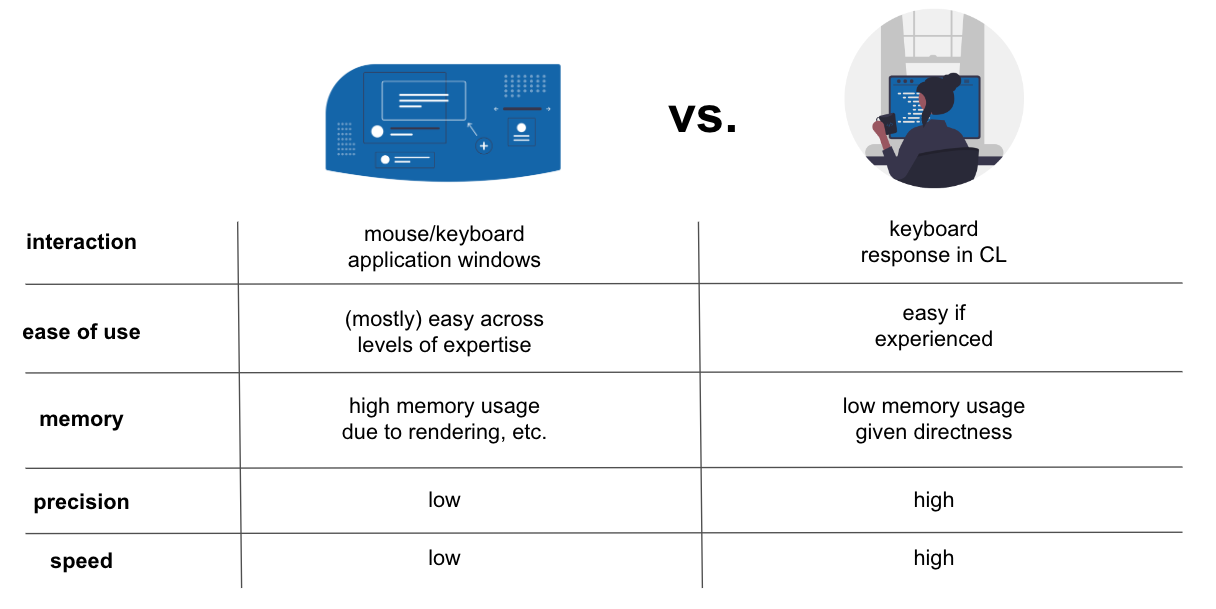
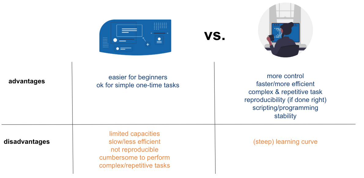
# * get to know important differences between `GUI`s & `CLI`s
# * learn basic and efficient usage of the `jupyter ecosystem` & `notebooks`
# * what is `Jupyter` & how to utilize `jupyter notebooks`
# ## GUI vs. CLI - interacting with machines
#
# ### You and your computer
#
#  # ### A little example
#
#
  #
#
#
# https://media4.giphy.com/media/l0HlO3BJ8LALPW4sE/giphy.gif?cid=790b7611adeaee8e2d808ee2724b8b2b3e1ba419871a5616&rid=giphy.gif&ct=g
# **We will dive right in!**
#
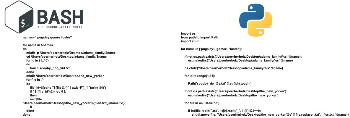
# Everyone gets 5 min to do the following:
#
# - create a `directory` structure (`folders`/`subfolders`) on your `desktop`
# `“addams_family/pugsley”`
# `“addams_family/gomez”`
# `“addams_family/fester”`
# - within each subfolder create `10 text files` called `“scooby_doo_[1-10].txt”`
# - move `text files` with `even numbers` to a new `folder` called `“the_new_yorker”` and add their origin `folder` to their name (e.g. `scooby_doo_2_pugsley.txt`)
#
# ### The frustration
#
#
#
#
#
# https://media4.giphy.com/media/l0HlO3BJ8LALPW4sE/giphy.gif?cid=790b7611adeaee8e2d808ee2724b8b2b3e1ba419871a5616&rid=giphy.gif&ct=g
# **We will dive right in!**
#
# Everyone gets 5 min to do the following:
#
# - create a `directory` structure (`folders`/`subfolders`) on your `desktop`
# `“addams_family/pugsley”`
# `“addams_family/gomez”`
# `“addams_family/fester”`
# - within each subfolder create `10 text files` called `“scooby_doo_[1-10].txt”`
# - move `text files` with `even numbers` to a new `folder` called `“the_new_yorker”` and add their origin `folder` to their name (e.g. `scooby_doo_2_pugsley.txt`)
#
# ### The frustration
#
#  #
#
#
# https://media4.giphy.com/media/l0HlO3BJ8LALPW4sE/giphy.gif?cid=790b7611adeaee8e2d808ee2724b8b2b3e1ba419871a5616&rid=giphy.gif&ct=g
# These tasks are anything but fun...now imagine you have to do this for hundreds of data samples/task/etc. … isn’t there a different way that is more feasible, faster, less prone to errors?
#
# Well, say no more!
# ### Why programming?
#
# Instead of the above task, or basically any other task manually, we can utilize `programming languages`, like `bash` and `python` to automate them. Thus, making them faster, less prone to errors and ideally reproducible.
#
#
#
#
#
#
# https://media4.giphy.com/media/l0HlO3BJ8LALPW4sE/giphy.gif?cid=790b7611adeaee8e2d808ee2724b8b2b3e1ba419871a5616&rid=giphy.gif&ct=g
# These tasks are anything but fun...now imagine you have to do this for hundreds of data samples/task/etc. … isn’t there a different way that is more feasible, faster, less prone to errors?
#
# Well, say no more!
# ### Why programming?
#
# Instead of the above task, or basically any other task manually, we can utilize `programming languages`, like `bash` and `python` to automate them. Thus, making them faster, less prone to errors and ideally reproducible.
#
#
#  #
#
#
#
#
#  #
#
#
# https://media1.giphy.com/media/Ld77zD3fF3Run8olIt/giphy.gif?cid=790b7611826db01ca8100bee189bbd8783d44c1090a1ca75&rid=giphy.gif&ct=g
# ### Still not convinced?
#
# Here some other `GUI`-based nightmares...
#
#
#
#
#
# https://media1.giphy.com/media/Ld77zD3fF3Run8olIt/giphy.gif?cid=790b7611826db01ca8100bee189bbd8783d44c1090a1ca75&rid=giphy.gif&ct=g
# ### Still not convinced?
#
# Here some other `GUI`-based nightmares...
#
#  #
# ### `GUI`vs. `CLI` - I
#
#
#
# ### `GUI`vs. `CLI` - I
#
#  #
# ### `GUI`vs. `CLI` - II
#
#
#
# ### `GUI`vs. `CLI` - II
#
#  #
# ### Where to program?
#
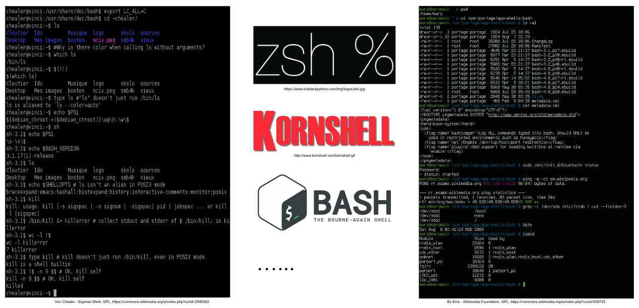
# #### The shell
#
#
#
# ### Where to program?
#
# #### The shell
#
#  #
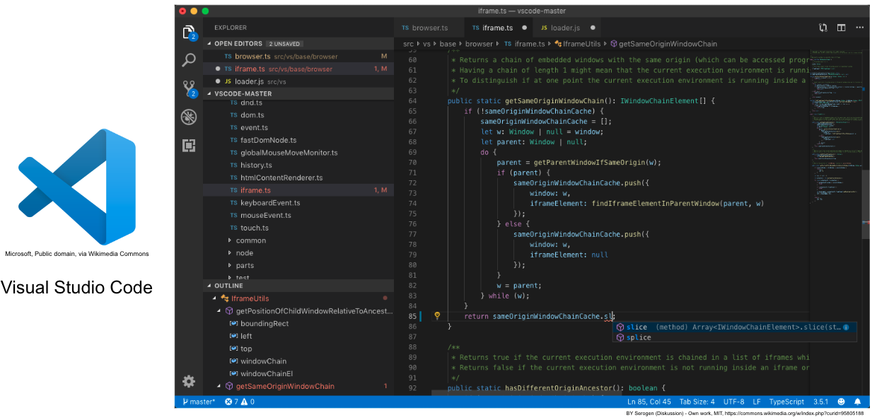
# #### Integrated development environment (IDEs)
#
# ##### General IDE
#
#
#
# #### Integrated development environment (IDEs)
#
# ##### General IDE
#
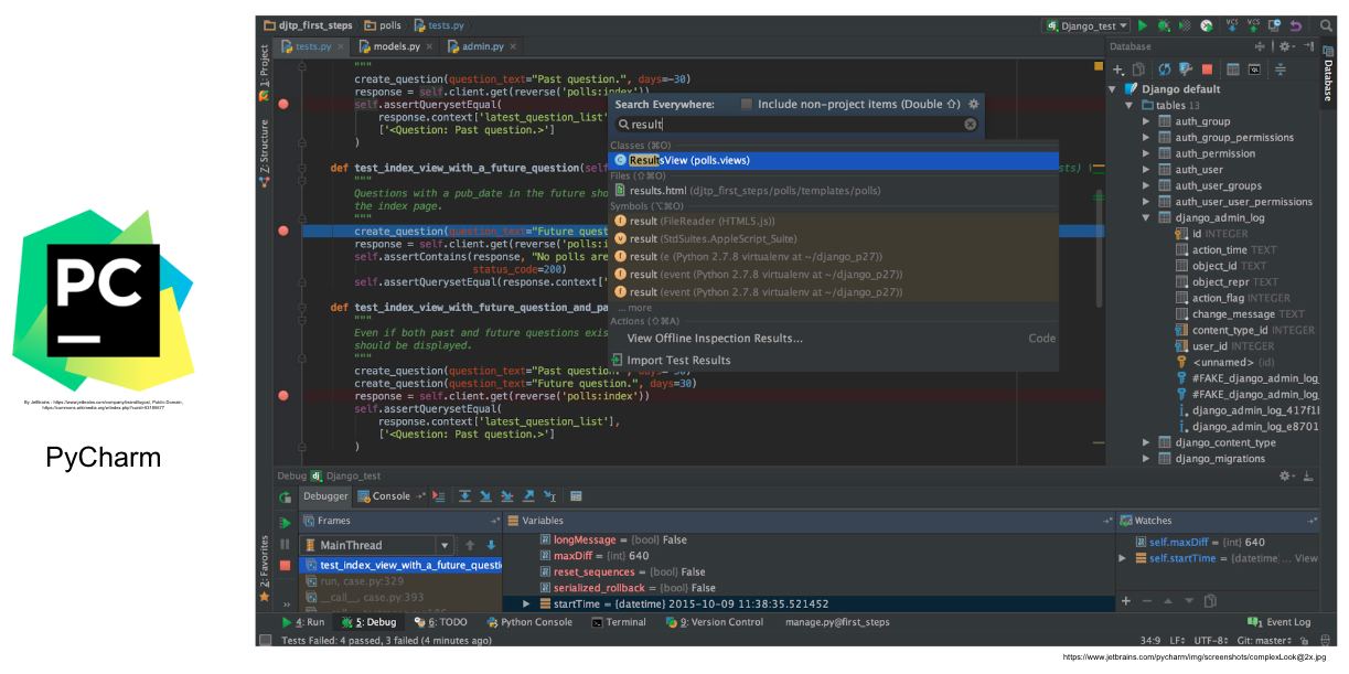
#  # ##### Language-specific IDE
#
#
  # ## To Jupyter & beyond
#
#
  #
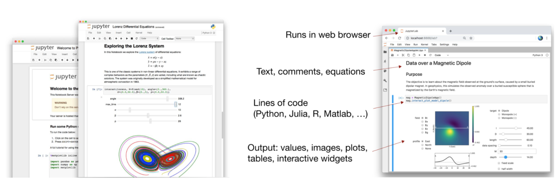
# - a community of people
#
# - an ecosystem of open tools and standards for interactive computing
#
# - language-agnostic and modular
#
# - empower people to use other open tools
#
# ## To Jupyter & beyond
#
#
#
# - a community of people
#
# - an ecosystem of open tools and standards for interactive computing
#
# - language-agnostic and modular
#
# - empower people to use other open tools
#
# ## To Jupyter & beyond
#
#  # ### Starting the notebook application/server
#
# 1. Open a terminal
# 2. Type `jupyter notebook`
# 3. If you're not automatically directed to a `webpage` copy the `URL` printed in the terminal and paste it in your `browser`
# ## Files Tab
#
# The `files tab` provides an interactive view of the portion of the `filesystem` which is accessible by the `user`. This is typically rooted by the directory in which the notebook server was started.
#
# The top of the `files list` displays `clickable` breadcrumbs of the `current directory`. It is possible to navigate the `filesystem` by clicking on these `breadcrumbs` or on the `directories` displayed in the `notebook list`.
#
# A new `notebook` can be created by clicking on the `New dropdown button` at the top of the list, and selecting the desired `language kernel`.
#
# `Notebooks` can also be `uploaded` to the `current directory` by dragging a `notebook` file onto the list or by clicking the `Upload button` at the top of the list.
# ### The Notebook
#
# When a `notebook` is opened, a new `browser tab` will be created which presents the `notebook user interface (UI)`. This `UI` allows for `interactively editing` and `running` the `notebook document`.
#
# A new `notebook` can be created from the `dashboard` by clicking on the `Files tab`, followed by the `New dropdown button`, and then selecting the `language` of choice for the `notebook`.
#
# An `interactive tour` of the `notebook UI` can be started by selecting `Help` -> `User Interface Tour` from the `notebook menu bar`.
# ### Header
#
# At the top of the `notebook document` is a `header` which contains the `notebook title`, a `menubar`, and `toolbar`. This `header` remains `fixed` at the top of the screen, even as the `body` of the `notebook` is `scrolled`. The `title` can be edited `in-place` (which renames the `notebook file`), and the `menubar` and `toolbar` contain a variety of actions which control `notebook navigation` and `document structure`.
#
#
  # ### Body
#
# The `body` of a `notebook` is composed of `cells`. Each `cell` contains either `markdown`, `code input`, `code output`, or `raw text`. `Cells` can be included in any order and edited at-will, allowing for a large amount of flexibility for constructing a narrative.
#
# - `Markdown cells` - These are used to build a `nicely formatted narrative` around the `code` in the document. The majority of this lesson is composed of `markdown cells`.
# - to get a `markdown cell` you can either select the `cell` and use `esc` + `m` or via `Cell -> cell type -> markdown`
#
#
  # - `Code cells` - These are used to define the `computational code` in the `document`. They come in `two forms`:
# - the `input cell` where the `user` types the `code` to be `executed`,
# - and the `output cell` which is the `representation` of the `executed code`. Depending on the `code`, this `representation` may be a `simple scalar value`, or something more complex like a `plot` or an `interactive widget`.
# - to get a `code cell` you can either select the `cell` and use `esc` + `y` or via `Cell -> cell type -> code`
#
#
#
  #
# - `Raw cells` - These are used when `text` needs to be included in `raw form`, without `execution` or `transformation`.
#
#
#
# - `Raw cells` - These are used when `text` needs to be included in `raw form`, without `execution` or `transformation`.
#
#  #
# ### Modality
#
# The `notebook user interface` is `modal`. This means that the `keyboard` behaves `differently` depending upon the `current mode` of the `notebook`. A `notebook` has `two modes`: `edit` and `command`.
#
# `Edit mode` is indicated by a `green cell border` and a `prompt` showing in the `editor area`. When a `cell` is in `edit mode`, you can type into the `cell`, like a `normal text editor`.
#
#
#
# ### Modality
#
# The `notebook user interface` is `modal`. This means that the `keyboard` behaves `differently` depending upon the `current mode` of the `notebook`. A `notebook` has `two modes`: `edit` and `command`.
#
# `Edit mode` is indicated by a `green cell border` and a `prompt` showing in the `editor area`. When a `cell` is in `edit mode`, you can type into the `cell`, like a `normal text editor`.
#
#  # `Command mode` is indicated by a `grey cell border`. When in `command mode`, the structure of the `notebook` can be modified as a whole, but the `text` in `individual cells` cannot be changed. Most importantly, the `keyboard` is `mapped` to a set of `shortcuts` for efficiently performing `notebook and cell actions`. For example, pressing `c` when in `command` mode, will `copy` the `current cell`; no modifier is needed.
#
#
  # ### Mouse navigation
#
# The `first concept` to understand in `mouse-based navigation` is that `cells` can be `selected by clicking on them`. The `currently selected cell` is indicated with a `grey` or `green border depending` on whether the `notebook` is in `edit or command mode`. Clicking inside a `cell`'s `editor area` will enter `edit mode`. Clicking on the `prompt` or the `output area` of a `cell` will enter `command mode`.
#
# The `second concept` to understand in `mouse-based navigation` is that `cell actions` usually apply to the `currently selected cell`. For example, to `run` the `code in a cell`, select it and then click the `Run button` in the `toolbar` or the `Cell` -> `Run` menu item. Similarly, to `copy` a `cell`, select it and then click the `copy selected cells button` in the `toolbar` or the `Edit` -> `Copy` menu item. With this simple pattern, it should be possible to perform nearly every `action` with the `mouse`.
#
# `Markdown cells` have one other `state` which can be `modified` with the `mouse`. These `cells` can either be `rendered` or `unrendered`. When they are `rendered`, a nice `formatted representation` of the `cell`'s `contents` will be presented. When they are `unrendered`, the `raw text source` of the `cell` will be presented. To `render` the `selected cell` with the `mouse`, click the `button` in the `toolbar` or the `Cell` -> `Run` menu item. To `unrender` the `selected cell`, `double click` on the `cell`.
# ### Keyboard Navigation
#
# The `modal user interface` of the `IPython Notebook` has been optimized for efficient `keyboard` usage. This is made possible by having `two different sets` of `keyboard shortcuts`: one set that is `active in edit mode` and another in `command mode`.
#
# The most important `keyboard shortcuts` are `Enter`, which enters `edit mode`, and `Esc`, which enters `command mode`.
#
# In `edit mode`, most of the `keyboard` is dedicated to `typing` into the `cell's editor`. Thus, in `edit mode` there are relatively `few shortcuts`. In `command mode`, the entire `keyboard` is available for `shortcuts`, so there are many more possibilities.
#
# The following images give an overview of the available `keyboard shortcuts`. These can viewed in the `notebook` at any time via the `Help` -> `Keyboard Shortcuts` menu item.
#
 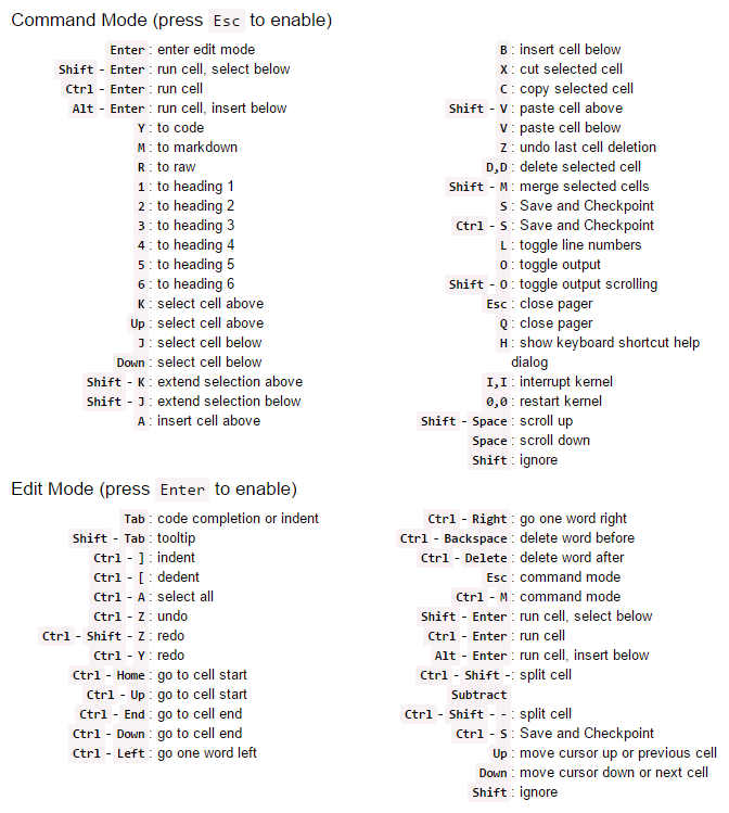 # The following shortcuts have been found to be the most useful in day-to-day tasks:
#
# - Basic navigation: `enter`, `shift-enter`, `up/k`, `down/j`
# - Saving the `notebook`: `s`
# - `Cell types`: `y`, `m`, `1-6`, `r`
# - `Cell creation`: `a`, `b`
# - `Cell editing`: `x`, `c`, `v`, `d`, `z`, `ctrl+shift+-`
# - `Kernel operations`: `i`, `.`
# ### Markdown Cells
#
# `Text` can be added to `IPython Notebooks` using `Markdown cells`. `Markdown` is a popular `markup language` that is a `superset of HTML`. Its specification can be found here:
#
# http://daringfireball.net/projects/markdown/
#
# You can view the `source` of a `cell` by `double clicking` on it, or while the `cell` is selected in `command mode`, press `Enter` to edit it. Once a `cell` has been `edited`, use `Shift-Enter` to `re-render` it.
# ### Markdown basics
#
# You can make text _italic_ or **bold**.
# You can build nested itemized or enumerated lists:
#
# * One
# - Sublist
# - This
# - Sublist
# - That
# - The other thing
# * Two
# - Sublist
# * Three
# - Sublist
# Now another list:
#
# 1. Here we go
# 1. Sublist
# 2. Sublist
# 2. There we go
# 3. Now this
# You can add horizontal rules:
#
# ---
# Here is a blockquote:
#
# > Beautiful is better than ugly.
# > Explicit is better than implicit.
# > Simple is better than complex.
# > Complex is better than complicated.
# > Flat is better than nested.
# > Sparse is better than dense.
# > Readability counts.
# > Special cases aren't special enough to break the rules.
# > Although practicality beats purity.
# > Errors should never pass silently.
# > Unless explicitly silenced.
# > In the face of ambiguity, refuse the temptation to guess.
# > There should be one-- and preferably only one --obvious way to do it.
# > Although that way may not be obvious at first unless you're Dutch.
# > Now is better than never.
# > Although never is often better than *right* now.
# > If the implementation is hard to explain, it's a bad idea.
# > If the implementation is easy to explain, it may be a good idea.
# > Namespaces are one honking great idea -- let's do more of those!
# You can add headings using Markdown's syntax:
#
#
# # Heading 1
#
# # Heading 2
#
# ## Heading 2.1
#
# ## Heading 2.2
#
# ### Embedded code
#
# You can embed code meant for illustration instead of execution in Python:
#
# def f(x):
# """a docstring"""
# return x**2
#
# or other languages:
#
# if (i=0; i
# ```python
# print "Hello World"
# ```
#
# ```javascript
# console.log("Hello World")
# ```
#
#
# Gives
# ```python
# print "Hello World"
# ```
#
# ```javascript
# console.log("Hello World")
# ```
# And a table like this :
#
#
# | This | is   |
# |------|------|
# |   a  | table|
#
#
# A nice HTML Table
#
# | This | is |
# |------|------|
# | a | table|
# ### General HTML
#
# Because `Markdown` is a `superset of HTML` you can even add things like `HTML tables`:
#
#
#
# | Header 1 |
# Header 2 |
#
#
# | row 1, cell 1 |
# row 1, cell 2 |
#
#
# | row 2, cell 1 |
# row 2, cell 2 |
#
#
# ### Local files
#
# If you have `local files` in your `Notebook directory`, you can refer to these `files` in `Markdown cells` directly:
#
# [subdirectory/]
# For example, in the `data` directory, we have the `jupyter ecosystem` graphic:
#
#  #
#
#
#  #
#
# These do not `embed` the data into the `notebook file`, and require that the `files` exist when you are viewing the `notebook`.
# ### Security of local files
#
# Note that this means that the `IPython notebook server` also acts as a `generic file server` for `files` inside the same `tree` as your `notebooks`. Access is not granted outside the `notebook` folder so you have strict control over what `files` are `visible`, but for this reason **it is highly recommended that you do not run the notebook server with a notebook directory at a high level in your filesystem (e.g. your home directory)**.
#
# When you run the `notebook` in a `password-protected` manner, `local file` access is `restricted` to `authenticated users` unless `read-only views` are active.
# ### Markdown attachments
#
# Since `Jupyter notebook version 5.0`, in addition to `referencing external files` you can `attach a file` to a `markdown cell`. To do so `drag` the `file` from e.g. the `browser` or local `storage` in a `markdown cell` while `editing` it:
#
# ``
#
#
# 
# `Files` are stored in `cell metadata` and will be `automatically scrubbed` at `save-time` if not `referenced`. You can recognize `attached images` from other `files` by their `url` that starts with `attachment`. For the `image` above:
#
# 
#
# Keep in mind that `attached files` will `increase the size` of your `notebook`.
#
# You can manually edit the `attachement` by using the `View` > `Cell Toolbar` > `Attachment` menu, but you should not need to.
# ### Code cells
#
# When executing code in `IPython`, all valid `Python syntax` works as-is, but `IPython` provides a number of `features` designed to make the `interactive experience` more `fluid` and `efficient`. First, we need to explain how to run `cells`. Try to run the `cell` below!
# In[1]:
import pandas as pd
print("Hi! This is a cell. Click on it and press the ▶ button above to run it")
# You can also run a cell with `Ctrl+Enter` or `Shift+Enter`. Experiment a bit with that.
# ### Tab Completion
#
# One of the most useful things about `Jupyter Notebook` is its tab completion.
#
# Try this: click just after `read_csv`( in the cell below and press `Shift+Tab` 4 times, slowly. Note that if you're using `JupyterLab` you don't have an additional help box option.
# In[ ]:
pd.read_csv(
# After the first time, you should see this:
#
#
#
#
# These do not `embed` the data into the `notebook file`, and require that the `files` exist when you are viewing the `notebook`.
# ### Security of local files
#
# Note that this means that the `IPython notebook server` also acts as a `generic file server` for `files` inside the same `tree` as your `notebooks`. Access is not granted outside the `notebook` folder so you have strict control over what `files` are `visible`, but for this reason **it is highly recommended that you do not run the notebook server with a notebook directory at a high level in your filesystem (e.g. your home directory)**.
#
# When you run the `notebook` in a `password-protected` manner, `local file` access is `restricted` to `authenticated users` unless `read-only views` are active.
# ### Markdown attachments
#
# Since `Jupyter notebook version 5.0`, in addition to `referencing external files` you can `attach a file` to a `markdown cell`. To do so `drag` the `file` from e.g. the `browser` or local `storage` in a `markdown cell` while `editing` it:
#
# ``
#
#
# 
# `Files` are stored in `cell metadata` and will be `automatically scrubbed` at `save-time` if not `referenced`. You can recognize `attached images` from other `files` by their `url` that starts with `attachment`. For the `image` above:
#
# 
#
# Keep in mind that `attached files` will `increase the size` of your `notebook`.
#
# You can manually edit the `attachement` by using the `View` > `Cell Toolbar` > `Attachment` menu, but you should not need to.
# ### Code cells
#
# When executing code in `IPython`, all valid `Python syntax` works as-is, but `IPython` provides a number of `features` designed to make the `interactive experience` more `fluid` and `efficient`. First, we need to explain how to run `cells`. Try to run the `cell` below!
# In[1]:
import pandas as pd
print("Hi! This is a cell. Click on it and press the ▶ button above to run it")
# You can also run a cell with `Ctrl+Enter` or `Shift+Enter`. Experiment a bit with that.
# ### Tab Completion
#
# One of the most useful things about `Jupyter Notebook` is its tab completion.
#
# Try this: click just after `read_csv`( in the cell below and press `Shift+Tab` 4 times, slowly. Note that if you're using `JupyterLab` you don't have an additional help box option.
# In[ ]:
pd.read_csv(
# After the first time, you should see this:
#
#  # After the second time:
#
#
 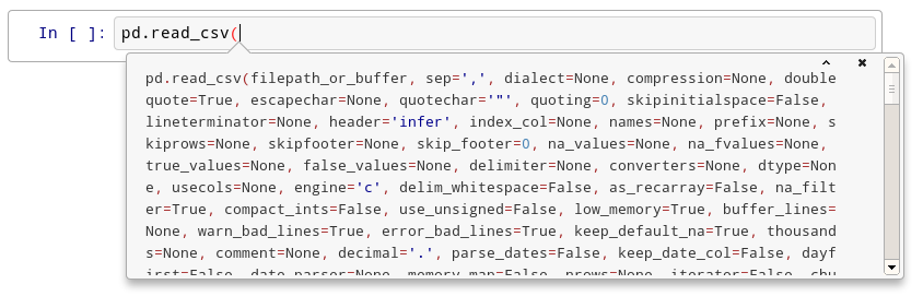 # After the fourth time, a big help box should pop up at the bottom of the screen, with the full documentation for the `read_csv` function:
#
#
  #
# This is amazingly useful. You can think of this as "the more confused I am, the more times I should press `Shift+Tab`".
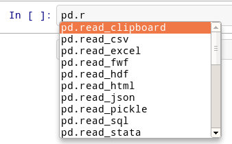
# Okay, let's try `tab completion` for `function names`!
# In[ ]:
pd.r
# You should see this:
#
#
#
# This is amazingly useful. You can think of this as "the more confused I am, the more times I should press `Shift+Tab`".
# Okay, let's try `tab completion` for `function names`!
# In[ ]:
pd.r
# You should see this:
#
#  # ## Get Help
#
# There's an additional way on how you can reach the help box shown above after the fourth `Shift+Tab` press. Instead, you can also use `obj`? or `obj`?? to get help or more help for an object.
# In[2]:
get_ipython().run_line_magic('pinfo', 'pd.read_csv')
# ## Writing code
#
# Writing code in a `notebook` is pretty normal.
# In[3]:
def print_10_nums():
for i in range(10):
print(i)
# In[4]:
print_10_nums()
# If you messed something up and want to revert to an older version of a code in a cell, use `Ctrl+Z` or to go than back `Ctrl+Y`.
#
# For a full list of all keyboard shortcuts, click on the small `keyboard icon` in the `notebook header` or click on `Help` > `Keyboard Shortcuts`.
# ### The interactive workflow: input, output, history
#
# `Notebooks` provide various options for `inputs` and `outputs`, while also allowing to access the `history` of `run commands`.
# In[5]:
2+10
# In[6]:
_+10
# You can suppress the `storage` and `rendering` of `output` if you append `;` to the last `cell` (this comes in handy when plotting with `matplotlib`, for example):
# In[7]:
10+20;
# In[8]:
_
# The `output` is stored in `_N` and `Out[N]` variables:
# In[9]:
_8 == Out[8]
# Previous inputs are available, too:
# In[10]:
In[9]
# In[11]:
_i
# In[12]:
get_ipython().run_line_magic('history', '-n 1-5')
# ### Accessing the underlying operating system
#
# Through `notebooks` you can also access the underlying `operating system` and `communicate` with it as you would do in e.g. a `terminal` via `bash`:
# In[1]:
get_ipython().system('pwd')
# In[2]:
files = get_ipython().getoutput('ls')
print("My current directory's files:")
print(files)
# In[3]:
get_ipython().system('echo $files')
# In[4]:
get_ipython().system('echo {files[0].upper()}')
# ### Magic functions
#
# `IPython` has all kinds of `magic functions`. `Magic functions` are prefixed by `%` or `%%,` and typically take their `arguments` without `parentheses`, `quotes` or even `commas` for convenience. `Line magics` take a single `%` and `cell magics` are prefixed with two `%%`.
# Some useful magic functions are:
#
# Magic Name | Effect
# ---------- | -------------------------------------------------------------
# %env | Get, set, or list environment variables
# %pdb | Control the automatic calling of the pdb interactive debugger
# %pylab | Load numpy and matplotlib to work interactively
# %%debug | Activates debugging mode in cell
# %%html | Render the cell as a block of HTML
# %%latex | Render the cell as a block of latex
# %%sh | %%sh script magic
# %%time | Time execution of a Python statement or expression
#
# You can run `%magic` to get a list of `magic functions` or `%quickref` for a reference sheet.
# In[17]:
get_ipython().run_line_magic('magic', '')
# `Line` vs `cell magics`:
# In[18]:
get_ipython().run_line_magic('timeit', 'list(range(1000))')
# In[19]:
get_ipython().run_cell_magic('timeit', '', 'list(range(10))\nlist(range(100))\n')
# `Line magics` can be used even inside `code blocks`:
# In[20]:
for i in range(1, 5):
size = i*100
print('size:', size, end=' ')
get_ipython().run_line_magic('timeit', 'list(range(size))')
# `Magics` can do anything they want with their input, so it doesn't have to be valid `Python`:
# In[21]:
get_ipython().run_cell_magic('bash', '', 'echo "My shell is:" $SHELL\necho "My disk usage is:"\ndf -h\n')
# Another interesting `cell magic`: create any `file` you want `locally` from the `notebook`:
# In[22]:
get_ipython().run_cell_magic('writefile', 'test.txt', 'This is a test file!\nIt can contain anything I want...\n\nAnd more...\n')
# In[23]:
get_ipython().system('cat test.txt')
# Let's see what other `magics` are currently defined in the `system`:
# In[24]:
get_ipython().run_line_magic('lsmagic', '')
# ## Writing latex
#
# Let's use `%%latex` to render a block of `latex`:
# In[25]:
get_ipython().run_cell_magic('latex', '', '$$F(k) = \\int_{-\\infty}^{\\infty} f(x) e^{2\\pi i k} \\mathrm{d} x$$\n')
# ### Running normal Python code: execution and errors
#
# Not only can you input normal `Python code`, you can even paste straight from a `Python` or `IPython shell session`:
# In[26]:
# Fibonacci series:
# the sum of two elements defines the next
a, b = 0, 1
while b < 10:
print(b)
a, b = b, a+b
# In[27]:
for i in range(10):
print(i, end=' ')
# And when your code produces errors, you can control how they are displayed with the `%xmode` magic:
# In[6]:
get_ipython().run_cell_magic('writefile', 'mod.py', '\ndef f(x):\n return 1.0/(x-1)\n\ndef g(y):\n return f(y+1)\n')
# Now let's call the function `g` with an argument that would produce an error:
# In[7]:
import mod
mod.g(0)
# In[8]:
get_ipython().run_line_magic('xmode', 'plain')
mod.g(0)
# In[9]:
get_ipython().run_line_magic('xmode', 'verbose')
mod.g(0)
# The default `%xmode` is "context", which shows additional context but not all local variables. Let's restore that one for the rest of our session.
# In[33]:
get_ipython().run_line_magic('xmode', 'context')
# ## Running code in other languages with special `%%` magics
# In[34]:
get_ipython().run_cell_magic('perl', '', '@months = ("July", "August", "September");\nprint $months[0];\n')
# In[35]:
get_ipython().run_cell_magic('ruby', '', 'name = "world"\nputs "Hello #{name.capitalize}!"\n')
# ### Raw Input in the notebook
#
# Since `1.0` the `IPython notebook web application` supports `raw_input` which for example allow us to invoke the `%debug` `magic` in the `notebook`:
# In[10]:
mod.g(0)
# In[11]:
get_ipython().run_line_magic('debug', '')
# Don't forget to exit your `debugging session`. `Raw input` can of course be used to ask for `user input`:
# In[38]:
enjoy = input('Are you enjoying this tutorial? ')
print('enjoy is:', enjoy)
# ### Plotting in the notebook
#
# `Notebooks` support a variety of fantastic `plotting options`, including `static` and `interactive` graphics. This `magic` configures `matplotlib` to `render` its `figures` `inline`:
# In[3]:
get_ipython().run_line_magic('matplotlib', 'inline')
# In[2]:
import numpy as np
import matplotlib.pyplot as plt
# In[41]:
x = np.linspace(0, 2*np.pi, 300)
y = np.sin(x**2)
plt.plot(x, y)
plt.title("A little chirp")
fig = plt.gcf() # let's keep the figure object around for later...
# In[2]:
import numpy as np
import plotly.figure_factory as ff
# Add histogram data
x1 = np.random.randn(200) - 2
x2 = np.random.randn(200)
x3 = np.random.randn(200) + 2
x4 = np.random.randn(200) + 4
# Group data together
hist_data = [x1, x2, x3, x4]
group_labels = ['Group 1', 'Group 2', 'Group 3', 'Group 4']
# Create distplot with custom bin_size
fig = ff.create_distplot(hist_data, group_labels, bin_size=.2)
fig.show()
# ### Interactive widgets
#
# `Jupyter notebooks` can also contain [interactive widgets](https://ipywidgets.readthedocs.io/en/latest/) that are great for `data exploration` and `visualization`. For example, we could explore the Lorenz System of Differential Equations (adapted from a [ipywidgets tutorial](https://ipywidgets.readthedocs.io/en/latest/)).
# In[3]:
from ipywidgets import interact, interactive
from IPython.display import clear_output, display, HTML
import numpy as np
from scipy import integrate
from matplotlib import pyplot as plt
from mpl_toolkits.mplot3d import Axes3D
from matplotlib.colors import cnames
from matplotlib import animation
def solve_lorenz(N=10, angle=0.0, max_time=4.0, sigma=10.0, beta=8./3, rho=28.0):
fig = plt.figure()
ax = fig.add_axes([0, 0, 1, 1], projection='3d')
ax.axis('off')
# prepare the axes limits
ax.set_xlim((-25, 25))
ax.set_ylim((-35, 35))
ax.set_zlim((5, 55))
def lorenz_deriv(x_y_z, t0, sigma=sigma, beta=beta, rho=rho):
"""Compute the time-derivative of a Lorenz system."""
x, y, z = x_y_z
return [sigma * (y - x), x * (rho - z) - y, x * y - beta * z]
# Choose random starting points, uniformly distributed from -15 to 15
np.random.seed(1)
x0 = -15 + 30 * np.random.random((N, 3))
# Solve for the trajectories
t = np.linspace(0, max_time, int(250*max_time))
x_t = np.asarray([integrate.odeint(lorenz_deriv, x0i, t)
for x0i in x0])
# choose a different color for each trajectory
colors = plt.cm.viridis(np.linspace(0, 1, N))
for i in range(N):
x, y, z = x_t[i,:,:].T
lines = ax.plot(x, y, z, '-', c=colors[i])
plt.setp(lines, linewidth=2)
ax.view_init(30, angle)
plt.show()
return t, x_t
# Having defined everything we need, we can now call our `interactive widget`!
# In[4]:
w = interactive(solve_lorenz, angle=(0.,360.), max_time=(0.1, 4.0),
N=(0,50), sigma=(0.0,50.0), rho=(0.0,50.0))
display(w)
# ### Taking things to the next level using `jupyter book`s
#
# All of the above discussed aspects and functionalities and many more can be nicely integrated with one another. The current pinnacle and most holistic outcome of this are [jupyter books](https://jupyterbook.org/en/stable/intro.html).
# In[7]:
from IPython.display import IFrame
IFrame(src='https://jupyterbook.org/en/stable/intro.html', width=1000, height=400)
# This makes them a great `framework` for **teaching workshops**
# In[8]:
IFrame(src='https://compneuro.neuromatch.io/tutorials/intro.html', width=1000, height=400)
# or **teaching courses/lectures**
# In[9]:
IFrame(src='https://peerherholz.github.io/Cog_Com_Neuro_ML_DL/index.html', width=1000, height=400)
# or **documenting workflows & analyses** for **interactive publications**
# In[10]:
IFrame(src='https://neuroscout.github.io/neuroscout-paper/intro.html', width=1000, height=400)
# In[11]:
IFrame(src='https://neurolibre.github.io/myelin-meta-analysis/intro.html', width=1000, height=400)
# ## The IPython kernel/client model
#
# Using the `jupyter notebook` we can actually interact with/adapt our `running` `kernel`.
# In[4]:
get_ipython().run_line_magic('connect_info', '')
# We can connect automatically a Qt Console to the currently running kernel with the `%qtconsole` magic, or by typing `ipython console --existing ` in any terminal:
# In[5]:
get_ipython().run_line_magic('qtconsole', '')
# ## Saving a Notebook
#
# `Jupyter Notebooks` `autosave`, so you don't have to worry about losing code too much. At the top of the page you can usually see the current save status:
#
# `Last Checkpoint: 2 minutes ago (unsaved changes)`
# `Last Checkpoint: a few seconds ago (autosaved)`
#
# If you want to save a notebook on purpose, either click on `File` > `Save` and `Checkpoint` or press `Ctrl+S`.
# ## To Jupyter & beyond
#
#
  #
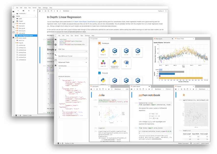
# - combining `code`, `data`, `visualization`, `text`, `interactive application` and much more types of content
# ### A whole new IDE: `Jupyter lab`
#
#
#
# - combining `code`, `data`, `visualization`, `text`, `interactive application` and much more types of content
# ### A whole new IDE: `Jupyter lab`
#
#  #
# Try it [here](https://jupyter.org/try-jupyter/lab/)!
#
# Try it [here](https://jupyter.org/try-jupyter/lab/)!

 # ### A little example
#
#

 #
#
#
#
#
# 


 # ### Body
#
# The `body` of a `notebook` is composed of `cells`. Each `cell` contains either `markdown`, `code input`, `code output`, or `raw text`. `Cells` can be included in any order and edited at-will, allowing for a large amount of flexibility for constructing a narrative.
#
# - `Markdown cells` - These are used to build a `nicely formatted narrative` around the `code` in the document. The majority of this lesson is composed of `markdown cells`.
# - to get a `markdown cell` you can either select the `cell` and use `esc` + `m` or via `Cell -> cell type -> markdown`
#
#
  # - `Code cells` - These are used to define the `computational code` in the `document`. They come in `two forms`:
# - the `input cell` where the `user` types the `code` to be `executed`,
# - and the `output cell` which is the `representation` of the `executed code`. Depending on the `code`, this `representation` may be a `simple scalar value`, or something more complex like a `plot` or an `interactive widget`.
# - to get a `code cell` you can either select the `cell` and use `esc` + `y` or via `Cell -> cell type -> code`
#
#
#
  #
# - `Raw cells` - These are used when `text` needs to be included in `raw form`, without `execution` or `transformation`.
#
#
#
# - `Raw cells` - These are used when `text` needs to be included in `raw form`, without `execution` or `transformation`.
#
#  #
# ### Modality
#
# The `notebook user interface` is `modal`. This means that the `keyboard` behaves `differently` depending upon the `current mode` of the `notebook`. A `notebook` has `two modes`: `edit` and `command`.
#
# `Edit mode` is indicated by a `green cell border` and a `prompt` showing in the `editor area`. When a `cell` is in `edit mode`, you can type into the `cell`, like a `normal text editor`.
#
#
#
# ### Modality
#
# The `notebook user interface` is `modal`. This means that the `keyboard` behaves `differently` depending upon the `current mode` of the `notebook`. A `notebook` has `two modes`: `edit` and `command`.
#
# `Edit mode` is indicated by a `green cell border` and a `prompt` showing in the `editor area`. When a `cell` is in `edit mode`, you can type into the `cell`, like a `normal text editor`.
#
#  # `Command mode` is indicated by a `grey cell border`. When in `command mode`, the structure of the `notebook` can be modified as a whole, but the `text` in `individual cells` cannot be changed. Most importantly, the `keyboard` is `mapped` to a set of `shortcuts` for efficiently performing `notebook and cell actions`. For example, pressing `c` when in `command` mode, will `copy` the `current cell`; no modifier is needed.
#
#
  # ### Mouse navigation
#
# The `first concept` to understand in `mouse-based navigation` is that `cells` can be `selected by clicking on them`. The `currently selected cell` is indicated with a `grey` or `green border depending` on whether the `notebook` is in `edit or command mode`. Clicking inside a `cell`'s `editor area` will enter `edit mode`. Clicking on the `prompt` or the `output area` of a `cell` will enter `command mode`.
#
# The `second concept` to understand in `mouse-based navigation` is that `cell actions` usually apply to the `currently selected cell`. For example, to `run` the `code in a cell`, select it and then click the `Run button` in the `toolbar` or the `Cell` -> `Run` menu item. Similarly, to `copy` a `cell`, select it and then click the `copy selected cells button` in the `toolbar` or the `Edit` -> `Copy` menu item. With this simple pattern, it should be possible to perform nearly every `action` with the `mouse`.
#
# `Markdown cells` have one other `state` which can be `modified` with the `mouse`. These `cells` can either be `rendered` or `unrendered`. When they are `rendered`, a nice `formatted representation` of the `cell`'s `contents` will be presented. When they are `unrendered`, the `raw text source` of the `cell` will be presented. To `render` the `selected cell` with the `mouse`, click the `button` in the `toolbar` or the `Cell` -> `Run` menu item. To `unrender` the `selected cell`, `double click` on the `cell`.
# ### Keyboard Navigation
#
# The `modal user interface` of the `IPython Notebook` has been optimized for efficient `keyboard` usage. This is made possible by having `two different sets` of `keyboard shortcuts`: one set that is `active in edit mode` and another in `command mode`.
#
# The most important `keyboard shortcuts` are `Enter`, which enters `edit mode`, and `Esc`, which enters `command mode`.
#
# In `edit mode`, most of the `keyboard` is dedicated to `typing` into the `cell's editor`. Thus, in `edit mode` there are relatively `few shortcuts`. In `command mode`, the entire `keyboard` is available for `shortcuts`, so there are many more possibilities.
#
# The following images give an overview of the available `keyboard shortcuts`. These can viewed in the `notebook` at any time via the `Help` -> `Keyboard Shortcuts` menu item.
#
  # The following shortcuts have been found to be the most useful in day-to-day tasks:
#
# - Basic navigation: `enter`, `shift-enter`, `up/k`, `down/j`
# - Saving the `notebook`: `s`
# - `Cell types`: `y`, `m`, `1-6`, `r`
# - `Cell creation`: `a`, `b`
# - `Cell editing`: `x`, `c`, `v`, `d`, `z`, `ctrl+shift+-`
# - `Kernel operations`: `i`, `.`
# ### Markdown Cells
#
# `Text` can be added to `IPython Notebooks` using `Markdown cells`. `Markdown` is a popular `markup language` that is a `superset of HTML`. Its specification can be found here:
#
# http://daringfireball.net/projects/markdown/
#
# You can view the `source` of a `cell` by `double clicking` on it, or while the `cell` is selected in `command mode`, press `Enter` to edit it. Once a `cell` has been `edited`, use `Shift-Enter` to `re-render` it.
# ### Markdown basics
#
# You can make text _italic_ or **bold**.
# You can build nested itemized or enumerated lists:
#
# * One
# - Sublist
# - This
# - Sublist
# - That
# - The other thing
# * Two
# - Sublist
# * Three
# - Sublist
# Now another list:
#
# 1. Here we go
# 1. Sublist
# 2. Sublist
# 2. There we go
# 3. Now this
# You can add horizontal rules:
#
# ---
# Here is a blockquote:
#
# > Beautiful is better than ugly.
# > Explicit is better than implicit.
# > Simple is better than complex.
# > Complex is better than complicated.
# > Flat is better than nested.
# > Sparse is better than dense.
# > Readability counts.
# > Special cases aren't special enough to break the rules.
# > Although practicality beats purity.
# > Errors should never pass silently.
# > Unless explicitly silenced.
# > In the face of ambiguity, refuse the temptation to guess.
# > There should be one-- and preferably only one --obvious way to do it.
# > Although that way may not be obvious at first unless you're Dutch.
# > Now is better than never.
# > Although never is often better than *right* now.
# > If the implementation is hard to explain, it's a bad idea.
# > If the implementation is easy to explain, it may be a good idea.
# > Namespaces are one honking great idea -- let's do more of those!
# You can add headings using Markdown's syntax:
#
#
  #
#
#
#  #
#
# These do not `embed` the data into the `notebook file`, and require that the `files` exist when you are viewing the `notebook`.
# ### Security of local files
#
# Note that this means that the `IPython notebook server` also acts as a `generic file server` for `files` inside the same `tree` as your `notebooks`. Access is not granted outside the `notebook` folder so you have strict control over what `files` are `visible`, but for this reason **it is highly recommended that you do not run the notebook server with a notebook directory at a high level in your filesystem (e.g. your home directory)**.
#
# When you run the `notebook` in a `password-protected` manner, `local file` access is `restricted` to `authenticated users` unless `read-only views` are active.
# ### Markdown attachments
#
# Since `Jupyter notebook version 5.0`, in addition to `referencing external files` you can `attach a file` to a `markdown cell`. To do so `drag` the `file` from e.g. the `browser` or local `storage` in a `markdown cell` while `editing` it:
#
# ``
#
#
# 
# `Files` are stored in `cell metadata` and will be `automatically scrubbed` at `save-time` if not `referenced`. You can recognize `attached images` from other `files` by their `url` that starts with `attachment`. For the `image` above:
#
# 
#
# Keep in mind that `attached files` will `increase the size` of your `notebook`.
#
# You can manually edit the `attachement` by using the `View` > `Cell Toolbar` > `Attachment` menu, but you should not need to.
# ### Code cells
#
# When executing code in `IPython`, all valid `Python syntax` works as-is, but `IPython` provides a number of `features` designed to make the `interactive experience` more `fluid` and `efficient`. First, we need to explain how to run `cells`. Try to run the `cell` below!
# In[1]:
import pandas as pd
print("Hi! This is a cell. Click on it and press the ▶ button above to run it")
# You can also run a cell with `Ctrl+Enter` or `Shift+Enter`. Experiment a bit with that.
# ### Tab Completion
#
# One of the most useful things about `Jupyter Notebook` is its tab completion.
#
# Try this: click just after `read_csv`( in the cell below and press `Shift+Tab` 4 times, slowly. Note that if you're using `JupyterLab` you don't have an additional help box option.
# In[ ]:
pd.read_csv(
# After the first time, you should see this:
#
#
#
#
# These do not `embed` the data into the `notebook file`, and require that the `files` exist when you are viewing the `notebook`.
# ### Security of local files
#
# Note that this means that the `IPython notebook server` also acts as a `generic file server` for `files` inside the same `tree` as your `notebooks`. Access is not granted outside the `notebook` folder so you have strict control over what `files` are `visible`, but for this reason **it is highly recommended that you do not run the notebook server with a notebook directory at a high level in your filesystem (e.g. your home directory)**.
#
# When you run the `notebook` in a `password-protected` manner, `local file` access is `restricted` to `authenticated users` unless `read-only views` are active.
# ### Markdown attachments
#
# Since `Jupyter notebook version 5.0`, in addition to `referencing external files` you can `attach a file` to a `markdown cell`. To do so `drag` the `file` from e.g. the `browser` or local `storage` in a `markdown cell` while `editing` it:
#
# ``
#
#
# 
# `Files` are stored in `cell metadata` and will be `automatically scrubbed` at `save-time` if not `referenced`. You can recognize `attached images` from other `files` by their `url` that starts with `attachment`. For the `image` above:
#
# 
#
# Keep in mind that `attached files` will `increase the size` of your `notebook`.
#
# You can manually edit the `attachement` by using the `View` > `Cell Toolbar` > `Attachment` menu, but you should not need to.
# ### Code cells
#
# When executing code in `IPython`, all valid `Python syntax` works as-is, but `IPython` provides a number of `features` designed to make the `interactive experience` more `fluid` and `efficient`. First, we need to explain how to run `cells`. Try to run the `cell` below!
# In[1]:
import pandas as pd
print("Hi! This is a cell. Click on it and press the ▶ button above to run it")
# You can also run a cell with `Ctrl+Enter` or `Shift+Enter`. Experiment a bit with that.
# ### Tab Completion
#
# One of the most useful things about `Jupyter Notebook` is its tab completion.
#
# Try this: click just after `read_csv`( in the cell below and press `Shift+Tab` 4 times, slowly. Note that if you're using `JupyterLab` you don't have an additional help box option.
# In[ ]:
pd.read_csv(
# After the first time, you should see this:
#
# 


 #
# - combining `code`, `data`, `visualization`, `text`, `interactive application` and much more types of content
# ### A whole new IDE: `Jupyter lab`
#
#
#
# - combining `code`, `data`, `visualization`, `text`, `interactive application` and much more types of content
# ### A whole new IDE: `Jupyter lab`
#
#  #
# Try it [here](https://jupyter.org/try-jupyter/lab/)!
#
# Try it [here](https://jupyter.org/try-jupyter/lab/)!