 #
#
# Another example of Vector Geometries is encountered when adding features to a visualization, such as Contents or Borders. The geometries of these features are drawn onto our screen.
#
#
#
#
#
#
# Another example of Vector Geometries is encountered when adding features to a visualization, such as Contents or Borders. The geometries of these features are drawn onto our screen.
#
#
#
#  #
#
# ### Shapely Example
# One Python package which is used for representing and manipulating geometries is [Shapely](https://shapely.readthedocs.io/en/stable/manual.html).
#
# Shapely can be paired with SpatialPandas and other packages to represent unstructured grid elements (nodes, edges, faces) as geometries for visualization.
#
# The following code snippets are basic examples of how these elements can be represented as geometries.
#
# In[1]:
import shapely as sp
# A node is represented as a pair of longitude and latitude coordinates
# In[2]:
sp.Point([0.0, 0.0])
# An edge is represented as a pair of nodes.
# In[3]:
sp.LineString([[0.0, 0.0], [180, -90]])
# A face is represented as a counter-clockwise set of nodes, with the first and final nodes in the set being equivalent (form a closed face)
# In[4]:
sp.Polygon([[100, 40], [100, 50], [90, 50], [90, 40], [100, 40]])
# ## Rasterization
#
# While there is definitely merit in rendering each geometric shape directly, this operation is computationally expensive for large datasets.
#
# Rasterization is a technique in computer graphics that converts vector (a.k.a geometric shapes) graphics into a raster image, which can be thought of as a regularly-sampled array of pixel values used for rendering.
#
# The figure below shows a simplified example of how rasterization "approximates" the geometry of different elements.
#
#
#
#
#
#
# ### Shapely Example
# One Python package which is used for representing and manipulating geometries is [Shapely](https://shapely.readthedocs.io/en/stable/manual.html).
#
# Shapely can be paired with SpatialPandas and other packages to represent unstructured grid elements (nodes, edges, faces) as geometries for visualization.
#
# The following code snippets are basic examples of how these elements can be represented as geometries.
#
# In[1]:
import shapely as sp
# A node is represented as a pair of longitude and latitude coordinates
# In[2]:
sp.Point([0.0, 0.0])
# An edge is represented as a pair of nodes.
# In[3]:
sp.LineString([[0.0, 0.0], [180, -90]])
# A face is represented as a counter-clockwise set of nodes, with the first and final nodes in the set being equivalent (form a closed face)
# In[4]:
sp.Polygon([[100, 40], [100, 50], [90, 50], [90, 40], [100, 40]])
# ## Rasterization
#
# While there is definitely merit in rendering each geometric shape directly, this operation is computationally expensive for large datasets.
#
# Rasterization is a technique in computer graphics that converts vector (a.k.a geometric shapes) graphics into a raster image, which can be thought of as a regularly-sampled array of pixel values used for rendering.
#
# The figure below shows a simplified example of how rasterization "approximates" the geometry of different elements.
#
#
#
#  #
#
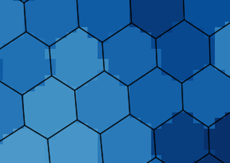
# For unstructured grids, rasterization looks something like the following.
#
#
#
#
#
#
# For unstructured grids, rasterization looks something like the following.
#
#
#
#  #
#
# The black edges outline the expected geometry of each face (a.k.a polygon).
#
# We can observe the jaggedness in the shading, which is the product of rasterization approximating each face.
#
#
#
# The black edges outline the expected geometry of each face (a.k.a polygon).
#
# We can observe the jaggedness in the shading, which is the product of rasterization approximating each face.
# Note:
# The selection between vector graphics and rasterization needs to be made taking into account several factors such as how large is the dataset (i.e. how fine-resolution the data is), what data fidelity with the visualization is desired, what performance is expected, etc. #See also:
# A more comprehensive showcase of rasterization can be found here #