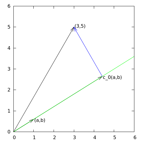
Approximation of a two-dimensional vector in a one-dimensional vector space.
# #
#
#
#
# We introduce the vector space $V$
# spanned by the vector $\boldsymbol{\psi}_0=(a,b)$:
#
#
#
# $$
# \begin{equation}
# V = \mbox{span}\,\{ \boldsymbol{\psi}_0\}{\thinspace .} \label{_auto1} \tag{2}
# \end{equation}
# $$
# We say that $\boldsymbol{\psi}_0$ is a *basis vector* in the space $V$.
# Our aim is to find the vector
#
#
#
# $$
# \begin{equation}
# \label{uc0} \tag{3}
# \boldsymbol{u} = c_0\boldsymbol{\psi}_0\in V
# \end{equation}
# $$
# which best approximates
# the given vector $\boldsymbol{f} = (3,5)$. A reasonable criterion for a best
# approximation could be to minimize the length of the difference between
# the approximate $\boldsymbol{u}$ and the given $\boldsymbol{f}$. The difference, or error
# $\boldsymbol{e} = \boldsymbol{f} -\boldsymbol{u}$, has its length given by the *norm*
# $$
# ||\boldsymbol{e}|| = (\boldsymbol{e},\boldsymbol{e})^{\frac{1}{2}},
# $$
# where $(\boldsymbol{e},\boldsymbol{e})$ is the *inner product* of $\boldsymbol{e}$ and itself. The inner
# product, also called *scalar product* or *dot product*, of two vectors
# $\boldsymbol{u}=(u_0,u_1)$ and $\boldsymbol{v} =(v_0,v_1)$ is defined as
#
#
#
# $$
# \begin{equation}
# (\boldsymbol{u}, \boldsymbol{v}) = u_0v_0 + u_1v_1{\thinspace .} \label{_auto2} \tag{4}
# \end{equation}
# $$
# **Remark.** We should point out that we use the notation
# $(\cdot,\cdot)$ for two different things: $(a,b)$ for scalar
# quantities $a$ and $b$ means the vector starting at the origin and
# ending in the point $(a,b)$, while $(\boldsymbol{u},\boldsymbol{v})$ with vectors $\boldsymbol{u}$ and
# $\boldsymbol{v}$ means the inner product of these vectors. Since vectors are here
# written in boldface font there should be no confusion. We may add
# that the norm associated with this inner product is the usual
# Euclidean length of a vector, i.e.,
# $$
# \|\boldsymbol{u}\| = \sqrt{(\boldsymbol{u},\boldsymbol{u})} = \sqrt{u_0^2 + u_1^2}
# $$
# ### The least squares method
#
# We now want to determine the $\boldsymbol{u}$ that minimizes $||\boldsymbol{e}||$, that is
# we want to compute the optimal $c_0$ in ([3](#uc0)). The algebra
# is simplified if we minimize the square of the norm, $||\boldsymbol{e}||^2 = (\boldsymbol{e}, \boldsymbol{e})$,
# instead of the norm itself.
# Define the function
#
#
#
# $$
# \begin{equation}
# E(c_0) = (\boldsymbol{e},\boldsymbol{e}) = (\boldsymbol{f} - c_0\boldsymbol{\psi}_0, \boldsymbol{f} - c_0\boldsymbol{\psi}_0)
# {\thinspace .}
# \label{_auto3} \tag{5}
# \end{equation}
# $$
# We can rewrite the expressions of the right-hand side in a more
# convenient form for further use:
#
#
#
# $$
# \begin{equation}
# E(c_0) = (\boldsymbol{f},\boldsymbol{f}) - 2c_0(\boldsymbol{f},\boldsymbol{\psi}_0) + c_0^2(\boldsymbol{\psi}_0,\boldsymbol{\psi}_0){\thinspace .}
# \label{fem:vec:E} \tag{6}
# \end{equation}
# $$
# This rewrite results from using the following fundamental rules for inner
# product spaces:
#
#
#
# $$
# \begin{equation}
# (\alpha\boldsymbol{u},\boldsymbol{v})=\alpha(\boldsymbol{u},\boldsymbol{v}),\quad \alpha\in\mathbb{R},
# \label{fem:vec:rule:scalarmult} \tag{7}
# \end{equation}
# $$
#
#
#
# $$
# \begin{equation}
# (\boldsymbol{u} +\boldsymbol{v},\boldsymbol{w}) = (\boldsymbol{u},\boldsymbol{w}) + (\boldsymbol{v}, \boldsymbol{w}),
# \label{fem:vec:rule:sum} \tag{8}
# \end{equation}
# $$
#
#
#
# $$
# \begin{equation}
# \label{fem:vec:rule:symmetry} \tag{9}
# (\boldsymbol{u}, \boldsymbol{v}) = (\boldsymbol{v}, \boldsymbol{u}){\thinspace .}
# \end{equation}
# $$
# Minimizing $E(c_0)$ implies finding $c_0$ such that
# $$
# \frac{\partial E}{\partial c_0} = 0{\thinspace .}
# $$
# It turns out that $E$ has one unique minimum and no maximum point.
# Now, when differentiating ([6](#fem:vec:E)) with respect to $c_0$, note
# that none of the inner product expressions depend on $c_0$, so we simply get
#
#
#
# $$
# \begin{equation}
# \frac{\partial E}{\partial c_0} = -2(\boldsymbol{f},\boldsymbol{\psi}_0) + 2c_0 (\boldsymbol{\psi}_0,\boldsymbol{\psi}_0)
# {\thinspace .}
# \label{fem:vec:dEdc0:v1} \tag{10}
# \end{equation}
# $$
# Setting the above expression equal to zero and solving for $c_0$ gives
#
#
#
# $$
# \begin{equation}
# c_0 = \frac{(\boldsymbol{f},\boldsymbol{\psi}_0)}{(\boldsymbol{\psi}_0,\boldsymbol{\psi}_0)},
# \label{fem:vec:c0} \tag{11}
# \end{equation}
# $$
# which in the present case, with $\boldsymbol{\psi}_0=(a,b)$, results in
#
#
#
# $$
# \begin{equation}
# c_0 = \frac{3a + 5b}{a^2 + b^2}{\thinspace .} \label{_auto4} \tag{12}
# \end{equation}
# $$
# For later, it is worth mentioning that setting
# the key equation ([10](#fem:vec:dEdc0:v1)) to zero and ordering
# the terms lead to
# $$
# (\boldsymbol{f}-c_0\boldsymbol{\psi}_0,\boldsymbol{\psi}_0) = 0,
# $$
# or
#
#
#
# $$
# \begin{equation}
# (\boldsymbol{e}, \boldsymbol{\psi}_0) = 0
# {\thinspace .}
# \label{fem:vec:dEdc0:Galerkin} \tag{13}
# \end{equation}
# $$
# This implication of minimizing $E$ is an important result that we shall
# make much use of.
#
#
#
#
# ### The projection method
#
# We shall now show that minimizing $||\boldsymbol{e}||^2$ implies that $\boldsymbol{e}$ is
# orthogonal to *any* vector $\boldsymbol{v}$ in the space $V$. This result is
# visually quite clear from [Figure](#fem:approx:vec:plane:fig) (think of
# other vectors along the line $(a,b)$: all of them will lead to
# a larger distance between the approximation and $\boldsymbol{f}$).
# Then we see mathematically that $\boldsymbol{e}$ is orthogonal to any vector $\boldsymbol{v}$
# in the space $V$ and we may
# express any $\boldsymbol{v}\in V$ as $\boldsymbol{v}=s\boldsymbol{\psi}_0$ for any scalar parameter $s$
# (recall that two vectors are orthogonal when their inner product vanishes).
# Then we calculate the inner product
# $$
# \begin{align*}
# (\boldsymbol{e}, s\boldsymbol{\psi}_0) &= (\boldsymbol{f} - c_0\boldsymbol{\psi}_0, s\boldsymbol{\psi}_0)\\
# &= (\boldsymbol{f},s\boldsymbol{\psi}_0) - (c_0\boldsymbol{\psi}_0, s\boldsymbol{\psi}_0)\\
# &= s(\boldsymbol{f},\boldsymbol{\psi}_0) - sc_0(\boldsymbol{\psi}_0, \boldsymbol{\psi}_0)\\
# &= s(\boldsymbol{f},\boldsymbol{\psi}_0) - s\frac{(\boldsymbol{f},\boldsymbol{\psi}_0)}{(\boldsymbol{\psi}_0,\boldsymbol{\psi}_0)}(\boldsymbol{\psi}_0,\boldsymbol{\psi}_0)\\
# &= s\left( (\boldsymbol{f},\boldsymbol{\psi}_0) - (\boldsymbol{f},\boldsymbol{\psi}_0)\right)\\
# &=0{\thinspace .}
# \end{align*}
# $$
# Therefore, instead of minimizing the square of the norm, we could
# demand that $\boldsymbol{e}$ is orthogonal to any vector in $V$, which in our present
# simple case amounts to a single vector only.
# This method is known as *projection*.
# (The approach can also be referred to as a Galerkin method as
# explained at the end of the section [Approximation of general vectors](#fem:approx:vec:Np1dim).)
#
# Mathematically, the projection method is stated
# by the equation
#
#
#
# $$
# \begin{equation}
# (\boldsymbol{e}, \boldsymbol{v}) = 0,\quad\forall\boldsymbol{v}\in V{\thinspace .}
# \label{fem:vec:Galerkin1} \tag{14}
# \end{equation}
# $$
# An arbitrary $\boldsymbol{v}\in V$ can be expressed as
# $s\boldsymbol{\psi}_0$, $s\in\mathbb{R}$, and therefore
# ([14](#fem:vec:Galerkin1)) implies
# $$
# (\boldsymbol{e},s\boldsymbol{\psi}_0) = s(\boldsymbol{e}, \boldsymbol{\psi}_0) = 0,
# $$
# which means that the error must be orthogonal to the basis vector in
# the space $V$:
# $$
# (\boldsymbol{e}, \boldsymbol{\psi}_0)=0\quad\hbox{or}\quad
# (\boldsymbol{f} - c_0\boldsymbol{\psi}_0, \boldsymbol{\psi}_0)=0,
# $$
# which is what we found in ([13](#fem:vec:dEdc0:Galerkin)) from
# the least squares computations.
#
#
#
#
# ## Approximation of general vectors
#
#
#
# Let us generalize the vector approximation from the previous section
# to vectors in spaces with arbitrary dimension. Given some vector $\boldsymbol{f}$,
# we want to find the best approximation to this vector in
# the space
# $$
# V = \hbox{span}\,\{\boldsymbol{\psi}_0,\ldots,\boldsymbol{\psi}_N\}
# {\thinspace .}
# $$
# We assume that the space has dimension $N+1$ and
# that *basis vectors* $\boldsymbol{\psi}_0,\ldots,\boldsymbol{\psi}_N$ are
# linearly independent so that none of them are redundant.
# Any vector $\boldsymbol{u}\in V$ can then be written as a linear combination
# of the basis vectors, i.e.,
# $$
# \boldsymbol{u} = \sum_{j=0}^N c_j\boldsymbol{\psi}_j,
# $$
# where $c_j\in\mathbb{R}$ are scalar coefficients to be determined.
#
# ### The least squares method
#
# Now we want to find $c_0,\ldots,c_N$, such that $\boldsymbol{u}$ is the best
# approximation to $\boldsymbol{f}$ in the sense that the distance (error)
# $\boldsymbol{e} = \boldsymbol{f} - \boldsymbol{u}$ is minimized. Again, we define
# the squared distance as a function of the free parameters
# $c_0,\ldots,c_N$,
# $$
# E(c_0,\ldots,c_N) = (\boldsymbol{e},\boldsymbol{e}) = (\boldsymbol{f} -\sum_jc_j\boldsymbol{\psi}_j,\boldsymbol{f} -\sum_jc_j\boldsymbol{\psi}_j)
# \nonumber
# $$
#
#
#
# $$
# \begin{equation}
# = (\boldsymbol{f},\boldsymbol{f}) - 2\sum_{j=0}^N c_j(\boldsymbol{f},\boldsymbol{\psi}_j) +
# \sum_{p=0}^N\sum_{q=0}^N c_pc_q(\boldsymbol{\psi}_p,\boldsymbol{\psi}_q){\thinspace .}
# \label{fem:vec:genE} \tag{15}
# \end{equation}
# $$
# Minimizing this $E$ with respect to the independent variables
# $c_0,\ldots,c_N$ is obtained by requiring
# $$
# \frac{\partial E}{\partial c_i} = 0,\quad i=0,\ldots,N
# {\thinspace .}
# $$
# The first term in ([15](#fem:vec:genE)) is independent of $c_i$, so its
# derivative vanishes.
# The second term in ([15](#fem:vec:genE)) is differentiated as follows:
#
#
#
# $$
# \begin{equation}
# \frac{\partial}{\partial c_i}
# 2\sum_{j=0}^N c_j(\boldsymbol{f},\boldsymbol{\psi}_j) = 2(\boldsymbol{f},\boldsymbol{\psi}_i),
# \label{_auto5} \tag{16}
# \end{equation}
# $$
# since the expression to be differentiated is a sum and only one term,
# $c_i(\boldsymbol{f},\boldsymbol{\psi}_i)$,
# contains $c_i$ (this term is linear in $c_i$).
# To understand this differentiation in detail,
# write out the sum specifically for,
# e.g, $N=3$ and $i=1$.
#
# The last term in ([15](#fem:vec:genE))
# is more tedious to differentiate. It can be wise to write out the
# double sum for $N=1$ and perform differentiation with respect to
# $c_0$ and $c_1$ to see the structure of the expression. Thereafter,
# one can generalize to an arbitrary $N$ and observe that
#
#
#
# $$
# \begin{equation}
# \frac{\partial}{\partial c_i}
# c_pc_q =
# \left\lbrace\begin{array}{ll}
# 0, & \hbox{ if } p\neq i\hbox{ and } q\neq i,\\
# c_q, & \hbox{ if } p=i\hbox{ and } q\neq i,\\
# c_p, & \hbox{ if } p\neq i\hbox{ and } q=i,\\
# 2c_i, & \hbox{ if } p=q= i{\thinspace .}\\
# \end{array}\right.
# \label{_auto6} \tag{17}
# \end{equation}
# $$
# Then
# $$
# \frac{\partial}{\partial c_i}
# \sum_{p=0}^N\sum_{q=0}^N c_pc_q(\boldsymbol{\psi}_p,\boldsymbol{\psi}_q)
# = \sum_{p=0, p\neq i}^N c_p(\boldsymbol{\psi}_p,\boldsymbol{\psi}_i)
# + \sum_{q=0, q\neq i}^N c_q(\boldsymbol{\psi}_i,\boldsymbol{\psi}_q)
# +2c_i(\boldsymbol{\psi}_i,\boldsymbol{\psi}_i){\thinspace .}
# $$
# Since each of the two sums is missing the term $c_i(\boldsymbol{\psi}_i,\boldsymbol{\psi}_i)$,
# we may split the very last term in two, to get exactly that "missing"
# term for each sum. This idea allows us to write
#
#
#
# $$
# \begin{equation}
# \frac{\partial}{\partial c_i}
# \sum_{p=0}^N\sum_{q=0}^N c_pc_q(\boldsymbol{\psi}_p,\boldsymbol{\psi}_q)
# = 2\sum_{j=0}^N c_i(\boldsymbol{\psi}_j,\boldsymbol{\psi}_i){\thinspace .}
# \label{_auto7} \tag{18}
# \end{equation}
# $$
# It then follows that setting
# $$
# \frac{\partial E}{\partial c_i} = 0,\quad i=0,\ldots,N,
# $$
# implies
# $$
# - 2(\boldsymbol{f},\boldsymbol{\psi}_i) + 2\sum_{j=0}^N c_i(\boldsymbol{\psi}_j,\boldsymbol{\psi}_i) = 0,\quad i=0,\ldots,N{\thinspace .}
# $$
# Moving the first term to the right-hand side shows that the equation is
# actually a *linear system* for the unknown parameters $c_0,\ldots,c_N$:
#
#
#
# $$
# \begin{equation}
# \sum_{j=0}^N A_{i,j} c_j = b_i, \quad i=0,\ldots,N,
# \label{fem:approx:vec:Np1dim:eqsys} \tag{19}
# \end{equation}
# $$
# where
#
#
#
# $$
# \begin{equation}
# A_{i,j} = (\boldsymbol{\psi}_i,\boldsymbol{\psi}_j),
# \label{_auto8} \tag{20}
# \end{equation}
# $$
#
#
#
# $$
# \begin{equation}
# b_i = (\boldsymbol{\psi}_i, \boldsymbol{f}){\thinspace .} \label{_auto9} \tag{21}
# \end{equation}
# $$
# We have changed the order of the two vectors in the inner
# product according to ([9](#fem:vec:rule:symmetry)):
# $$
# A_{i,j} = (\boldsymbol{\psi}_j,\boldsymbol{\psi}_i) = (\boldsymbol{\psi}_i,\boldsymbol{\psi}_j),
# $$
# simply because the sequence $i$-$j$ looks more aesthetic.
#
# ### The Galerkin or projection method
#
# In analogy with the "one-dimensional" example in
# the section [Approximation of planar vectors](#fem:approx:vec:plane), it holds also here in the general
# case that minimizing the distance
# (error) $\boldsymbol{e}$ is equivalent to demanding that $\boldsymbol{e}$ is orthogonal to
# all $\boldsymbol{v}\in V$:
#
#
#
# $$
# \begin{equation}
# (\boldsymbol{e},\boldsymbol{v})=0,\quad \forall\boldsymbol{v}\in V{\thinspace .}
# \label{fem:approx:vec:Np1dim:Galerkin} \tag{22}
# \end{equation}
# $$
# Since any $\boldsymbol{v}\in V$ can be written as $\boldsymbol{v} =\sum_{i=0}^N c_i\boldsymbol{\psi}_i$,
# the statement ([22](#fem:approx:vec:Np1dim:Galerkin)) is equivalent to
# saying that
# $$
# (\boldsymbol{e}, \sum_{i=0}^N c_i\boldsymbol{\psi}_i) = 0,
# $$
# for any choice of coefficients $c_0,\ldots,c_N$.
# The latter equation can be rewritten as
# $$
# \sum_{i=0}^N c_i (\boldsymbol{e},\boldsymbol{\psi}_i) =0{\thinspace .}
# $$
# If this is to hold for arbitrary values of $c_0,\ldots,c_N$,
# we must require that each term in the sum vanishes, which means that
#
#
#
# $$
# \begin{equation}
# (\boldsymbol{e},\boldsymbol{\psi}_i)=0,\quad i=0,\ldots,N{\thinspace .}
# \label{fem:approx:vec:Np1dim:Galerkin0} \tag{23}
# \end{equation}
# $$
# These $N+1$ equations result in the same linear system as
# ([19](#fem:approx:vec:Np1dim:eqsys)):
# $$
# (\boldsymbol{f} - \sum_{j=0}^N c_j\boldsymbol{\psi}_j, \boldsymbol{\psi}_i) = (\boldsymbol{f}, \boldsymbol{\psi}_i) - \sum_{j=0}^N
# (\boldsymbol{\psi}_i,\boldsymbol{\psi}_j)c_j = 0,
# $$
# and hence
# $$
# \sum_{j=0}^N (\boldsymbol{\psi}_i,\boldsymbol{\psi}_j)c_j = (\boldsymbol{f}, \boldsymbol{\psi}_i),\quad i=0,\ldots, N
# {\thinspace .}
# $$
# So, instead of differentiating the
# $E(c_0,\ldots,c_N)$ function, we could simply use
# ([22](#fem:approx:vec:Np1dim:Galerkin)) as the principle for
# determining $c_0,\ldots,c_N$, resulting in the $N+1$
# equations ([23](#fem:approx:vec:Np1dim:Galerkin0)).
#
# The names *least squares method* or *least squares approximation*
# are natural since the calculations consists of
# minimizing $||\boldsymbol{e}||^2$, and $||\boldsymbol{e}||^2$ is a sum of squares
# of differences between the components in $\boldsymbol{f}$ and $\boldsymbol{u}$.
# We find $\boldsymbol{u}$ such that this sum of squares is minimized.
#
# The principle ([22](#fem:approx:vec:Np1dim:Galerkin)),
# or the equivalent form ([23](#fem:approx:vec:Np1dim:Galerkin0)),
# is known as *projection*. Almost the same mathematical idea
# was used by the Russian mathematician [Boris Galerkin](http://en.wikipedia.org/wiki/Boris_Galerkin) to solve
# differential equations, resulting in what is widely known as
# *Galerkin's method*.
#
# # Approximation principles
#
#
# Let $V$ be a function space spanned by a set of *basis functions*
# ${\psi}_0,\ldots,{\psi}_N$,
# $$
# V = \hbox{span}\,\{{\psi}_0,\ldots,{\psi}_N\},
# $$
# such that any function $u\in V$ can be written as a linear
# combination of the basis functions:
#
#
#
# $$
# \begin{equation}
# \label{fem:approx:ufem} \tag{24}
# u = \sum_{j\in{\mathcal{I}_s}} c_j{\psi}_j{\thinspace .}
# \end{equation}
# $$
# That is, we consider functions as vectors in a vector space - a
# so-called function space - and we have a finite set of basis
# functions that span the space just as basis vectors or unit vectors
# span a vector space.
#
# The index set ${\mathcal{I}_s}$ is defined as ${\mathcal{I}_s} =\{0,\ldots,N\}$ and is
# from now on used
# both for compact notation and for flexibility in the numbering of
# elements in sequences.
#
# For now, in this introduction, we shall look at functions of a
# single variable $x$:
# $u=u(x)$, ${\psi}_j={\psi}_j(x)$, $j\in{\mathcal{I}_s}$. Later, we will almost
# trivially extend the mathematical details
# to functions of two- or three-dimensional physical spaces.
# The approximation ([24](#fem:approx:ufem)) is typically used
# to discretize a problem in space. Other methods, most notably
# finite differences, are common for time discretization, although the
# form ([24](#fem:approx:ufem)) can be used in time as well.
#
# ## The least squares method
#
#
# Given a function $f(x)$, how can we determine its best approximation
# $u(x)\in V$? A natural starting point is to apply the same reasoning
# as we did for vectors in the section [Approximation of general vectors](#fem:approx:vec:Np1dim). That is,
# we minimize the distance between $u$ and $f$. However, this requires
# a norm for measuring distances, and a norm is most conveniently
# defined through an
# inner product. Viewing a function as a vector of infinitely
# many point values, one for each value of $x$, the inner product of
# two arbitrary functions $f(x)$ and $g(x)$ could
# intuitively be defined as the usual summation of
# pairwise "components" (values), with summation replaced by integration:
# $$
# (f,g) = \int f(x)g(x)\, {\, \mathrm{d}x}
# {\thinspace .}
# $$
# To fix the integration domain, we let $f(x)$ and ${\psi}_i(x)$
# be defined for a domain $\Omega\subset\mathbb{R}$.
# The inner product of two functions $f(x)$ and $g(x)$ is then
#
#
#
# $$
# \begin{equation}
# (f,g) = \int_\Omega f(x)g(x)\, {\, \mathrm{d}x}
# \label{fem:approx:LS:innerprod} \tag{25}
# {\thinspace .}
# \end{equation}
# $$
# The distance between $f$ and any function $u\in V$ is simply
# $f-u$, and the squared norm of this distance is
#
#
#
# $$
# \begin{equation}
# E = (f(x)-\sum_{j\in{\mathcal{I}_s}} c_j{\psi}_j(x), f(x)-\sum_{j\in{\mathcal{I}_s}} c_j{\psi}_j(x)){\thinspace .}
# \label{fem:approx:LS:E} \tag{26}
# \end{equation}
# $$
# Note the analogy with ([15](#fem:vec:genE)): the given function
# $f$ plays the role of the given vector $\boldsymbol{f}$, and the basis function
# ${\psi}_i$ plays the role of the basis vector $\boldsymbol{\psi}_i$.
# We can rewrite ([26](#fem:approx:LS:E)),
# through similar steps as used for the result
# ([15](#fem:vec:genE)), leading to
#
#
#
# $$
# \begin{equation}
# E(c_i, \ldots, c_N) = (f,f) -2\sum_{j\in{\mathcal{I}_s}} c_j(f,{\psi}_i)
# + \sum_{p\in{\mathcal{I}_s}}\sum_{q\in{\mathcal{I}_s}} c_pc_q({\psi}_p,{\psi}_q){\thinspace .} \label{_auto10} \tag{27}
# \end{equation}
# $$
# Minimizing this function of $N+1$ scalar variables
# $\left\{ {c}_i \right\}_{i\in{\mathcal{I}_s}}$, requires differentiation
# with respect to $c_i$, for all $i\in{\mathcal{I}_s}$. The resulting
# equations are very similar to those we had in the vector case,
# and we hence end up with a
# linear system of the form ([19](#fem:approx:vec:Np1dim:eqsys)), with
# basically the same expressions:
#
#
#
# $$
# \begin{equation}
# A_{i,j} = ({\psi}_i,{\psi}_j),
# \label{fem:approx:Aij} \tag{28}
# \end{equation}
# $$
#
#
#
# $$
# \begin{equation}
# b_i = (f,{\psi}_i){\thinspace .}
# \label{fem:approx:bi} \tag{29}
# \end{equation}
# $$
# The only difference from
# ([19](#fem:approx:vec:Np1dim:eqsys))
# is that the inner product is defined in terms
# of integration rather than summation.
#
# ## The projection (or Galerkin) method
#
#
# As in the section [Approximation of general vectors](#fem:approx:vec:Np1dim), the minimization of $(e,e)$
# is equivalent to
#
#
#
# $$
# \begin{equation}
# (e,v)=0,\quad\forall v\in V{\thinspace .}
# \label{fem:approx:Galerkin} \tag{30}
# \end{equation}
# $$
# This is known as a projection of a function $f$ onto the subspace $V$.
# We may also call it a Galerkin method for approximating functions.
# Using the same reasoning as
# in
# ([22](#fem:approx:vec:Np1dim:Galerkin))-([23](#fem:approx:vec:Np1dim:Galerkin0)),
# it follows that ([30](#fem:approx:Galerkin)) is equivalent to
#
#
#
# $$
# \begin{equation}
# (e,{\psi}_i)=0,\quad i\in{\mathcal{I}_s}{\thinspace .}
# \label{fem:approx:Galerkin0} \tag{31}
# \end{equation}
# $$
# Inserting $e=f-u$ in this equation and ordering terms, as in the
# multi-dimensional vector case, we end up with a linear
# system with a coefficient matrix ([28](#fem:approx:Aij)) and
# right-hand side vector ([29](#fem:approx:bi)).
#
# Whether we work with vectors in the plane, general vectors, or
# functions in function spaces, the least squares principle and
# the projection or Galerkin method are equivalent.
#
# ## Example of linear approximation
#
#
# Let us apply the theory in the previous section to a simple problem:
# given a parabola $f(x)=10(x-1)^2-1$ for $x\in\Omega=[1,2]$, find
# the best approximation $u(x)$ in the space of all linear functions:
# $$
# V = \hbox{span}\,\{1, x\}{\thinspace .}
# $$
# With our notation, ${\psi}_0(x)=1$, ${\psi}_1(x)=x$, and $N=1$.
# We seek
# $$
# u=c_0{\psi}_0(x) + c_1{\psi}_1(x) = c_0 + c_1x,
# $$
# where
# $c_0$ and $c_1$ are found by solving a $2\times 2$ linear system.
# The coefficient matrix has elements
#
#
#
# $$
# \begin{equation}
# A_{0,0} = ({\psi}_0,{\psi}_0) = \int_1^21\cdot 1\, {\, \mathrm{d}x} = 1,
# \label{_auto11} \tag{32}
# \end{equation}
# $$
#
#
#
# $$
# \begin{equation}
# A_{0,1} = ({\psi}_0,{\psi}_1) = \int_1^2 1\cdot x\, {\, \mathrm{d}x} = 3/2,
# \label{_auto12} \tag{33}
# \end{equation}
# $$
#
#
#
# $$
# \begin{equation}
# A_{1,0} = A_{0,1} = 3/2,
# \label{_auto13} \tag{34}
# \end{equation}
# $$
#
#
#
# $$
# \begin{equation}
# A_{1,1} = ({\psi}_1,{\psi}_1) = \int_1^2 x\cdot x\,{\, \mathrm{d}x} = 7/3{\thinspace .} \label{_auto14} \tag{35}
# \end{equation}
# $$
# The corresponding right-hand side is
#
#
#
# $$
# \begin{equation}
# b_1 = (f,{\psi}_0) = \int_1^2 (10(x-1)^2 - 1)\cdot 1 \, {\, \mathrm{d}x} = 7/3,
# \label{_auto15} \tag{36}
# \end{equation}
# $$
#
#
#
# $$
# \begin{equation}
# b_2 = (f,{\psi}_1) = \int_1^2 (10(x-1)^2 - 1)\cdot x\, {\, \mathrm{d}x} = 13/3{\thinspace .} \label{_auto16} \tag{37}
# \end{equation}
# $$
# Solving the linear system results in
#
#
#
# $$
# \begin{equation}
# c_0 = -38/3,\quad c_1 = 10,
# \label{_auto17} \tag{38}
# \end{equation}
# $$
# and consequently
#
#
#
# $$
# \begin{equation}
# u(x) = 10x - \frac{38}{3}{\thinspace .} \label{_auto18} \tag{39}
# \end{equation}
# $$
# [Figure](#fem:approx:global:fig:parabola:linear) displays the
# parabola and its best approximation in the space of all linear functions.
#
#
#
#
#
#
#
#
#
#
# We introduce the vector space $V$
# spanned by the vector $\boldsymbol{\psi}_0=(a,b)$:
#
#
#
# $$
# \begin{equation}
# V = \mbox{span}\,\{ \boldsymbol{\psi}_0\}{\thinspace .} \label{_auto1} \tag{2}
# \end{equation}
# $$
# We say that $\boldsymbol{\psi}_0$ is a *basis vector* in the space $V$.
# Our aim is to find the vector
#
#
#
# $$
# \begin{equation}
# \label{uc0} \tag{3}
# \boldsymbol{u} = c_0\boldsymbol{\psi}_0\in V
# \end{equation}
# $$
# which best approximates
# the given vector $\boldsymbol{f} = (3,5)$. A reasonable criterion for a best
# approximation could be to minimize the length of the difference between
# the approximate $\boldsymbol{u}$ and the given $\boldsymbol{f}$. The difference, or error
# $\boldsymbol{e} = \boldsymbol{f} -\boldsymbol{u}$, has its length given by the *norm*
# $$
# ||\boldsymbol{e}|| = (\boldsymbol{e},\boldsymbol{e})^{\frac{1}{2}},
# $$
# where $(\boldsymbol{e},\boldsymbol{e})$ is the *inner product* of $\boldsymbol{e}$ and itself. The inner
# product, also called *scalar product* or *dot product*, of two vectors
# $\boldsymbol{u}=(u_0,u_1)$ and $\boldsymbol{v} =(v_0,v_1)$ is defined as
#
#
#
# $$
# \begin{equation}
# (\boldsymbol{u}, \boldsymbol{v}) = u_0v_0 + u_1v_1{\thinspace .} \label{_auto2} \tag{4}
# \end{equation}
# $$
# **Remark.** We should point out that we use the notation
# $(\cdot,\cdot)$ for two different things: $(a,b)$ for scalar
# quantities $a$ and $b$ means the vector starting at the origin and
# ending in the point $(a,b)$, while $(\boldsymbol{u},\boldsymbol{v})$ with vectors $\boldsymbol{u}$ and
# $\boldsymbol{v}$ means the inner product of these vectors. Since vectors are here
# written in boldface font there should be no confusion. We may add
# that the norm associated with this inner product is the usual
# Euclidean length of a vector, i.e.,
# $$
# \|\boldsymbol{u}\| = \sqrt{(\boldsymbol{u},\boldsymbol{u})} = \sqrt{u_0^2 + u_1^2}
# $$
# ### The least squares method
#
# We now want to determine the $\boldsymbol{u}$ that minimizes $||\boldsymbol{e}||$, that is
# we want to compute the optimal $c_0$ in ([3](#uc0)). The algebra
# is simplified if we minimize the square of the norm, $||\boldsymbol{e}||^2 = (\boldsymbol{e}, \boldsymbol{e})$,
# instead of the norm itself.
# Define the function
#
#
#
# $$
# \begin{equation}
# E(c_0) = (\boldsymbol{e},\boldsymbol{e}) = (\boldsymbol{f} - c_0\boldsymbol{\psi}_0, \boldsymbol{f} - c_0\boldsymbol{\psi}_0)
# {\thinspace .}
# \label{_auto3} \tag{5}
# \end{equation}
# $$
# We can rewrite the expressions of the right-hand side in a more
# convenient form for further use:
#
#
#
# $$
# \begin{equation}
# E(c_0) = (\boldsymbol{f},\boldsymbol{f}) - 2c_0(\boldsymbol{f},\boldsymbol{\psi}_0) + c_0^2(\boldsymbol{\psi}_0,\boldsymbol{\psi}_0){\thinspace .}
# \label{fem:vec:E} \tag{6}
# \end{equation}
# $$
# This rewrite results from using the following fundamental rules for inner
# product spaces:
#
#
#
# $$
# \begin{equation}
# (\alpha\boldsymbol{u},\boldsymbol{v})=\alpha(\boldsymbol{u},\boldsymbol{v}),\quad \alpha\in\mathbb{R},
# \label{fem:vec:rule:scalarmult} \tag{7}
# \end{equation}
# $$
#
#
#
# $$
# \begin{equation}
# (\boldsymbol{u} +\boldsymbol{v},\boldsymbol{w}) = (\boldsymbol{u},\boldsymbol{w}) + (\boldsymbol{v}, \boldsymbol{w}),
# \label{fem:vec:rule:sum} \tag{8}
# \end{equation}
# $$
#
#
#
# $$
# \begin{equation}
# \label{fem:vec:rule:symmetry} \tag{9}
# (\boldsymbol{u}, \boldsymbol{v}) = (\boldsymbol{v}, \boldsymbol{u}){\thinspace .}
# \end{equation}
# $$
# Minimizing $E(c_0)$ implies finding $c_0$ such that
# $$
# \frac{\partial E}{\partial c_0} = 0{\thinspace .}
# $$
# It turns out that $E$ has one unique minimum and no maximum point.
# Now, when differentiating ([6](#fem:vec:E)) with respect to $c_0$, note
# that none of the inner product expressions depend on $c_0$, so we simply get
#
#
#
# $$
# \begin{equation}
# \frac{\partial E}{\partial c_0} = -2(\boldsymbol{f},\boldsymbol{\psi}_0) + 2c_0 (\boldsymbol{\psi}_0,\boldsymbol{\psi}_0)
# {\thinspace .}
# \label{fem:vec:dEdc0:v1} \tag{10}
# \end{equation}
# $$
# Setting the above expression equal to zero and solving for $c_0$ gives
#
#
#
# $$
# \begin{equation}
# c_0 = \frac{(\boldsymbol{f},\boldsymbol{\psi}_0)}{(\boldsymbol{\psi}_0,\boldsymbol{\psi}_0)},
# \label{fem:vec:c0} \tag{11}
# \end{equation}
# $$
# which in the present case, with $\boldsymbol{\psi}_0=(a,b)$, results in
#
#
#
# $$
# \begin{equation}
# c_0 = \frac{3a + 5b}{a^2 + b^2}{\thinspace .} \label{_auto4} \tag{12}
# \end{equation}
# $$
# For later, it is worth mentioning that setting
# the key equation ([10](#fem:vec:dEdc0:v1)) to zero and ordering
# the terms lead to
# $$
# (\boldsymbol{f}-c_0\boldsymbol{\psi}_0,\boldsymbol{\psi}_0) = 0,
# $$
# or
#
#
#
# $$
# \begin{equation}
# (\boldsymbol{e}, \boldsymbol{\psi}_0) = 0
# {\thinspace .}
# \label{fem:vec:dEdc0:Galerkin} \tag{13}
# \end{equation}
# $$
# This implication of minimizing $E$ is an important result that we shall
# make much use of.
#
#
#
#
# ### The projection method
#
# We shall now show that minimizing $||\boldsymbol{e}||^2$ implies that $\boldsymbol{e}$ is
# orthogonal to *any* vector $\boldsymbol{v}$ in the space $V$. This result is
# visually quite clear from [Figure](#fem:approx:vec:plane:fig) (think of
# other vectors along the line $(a,b)$: all of them will lead to
# a larger distance between the approximation and $\boldsymbol{f}$).
# Then we see mathematically that $\boldsymbol{e}$ is orthogonal to any vector $\boldsymbol{v}$
# in the space $V$ and we may
# express any $\boldsymbol{v}\in V$ as $\boldsymbol{v}=s\boldsymbol{\psi}_0$ for any scalar parameter $s$
# (recall that two vectors are orthogonal when their inner product vanishes).
# Then we calculate the inner product
# $$
# \begin{align*}
# (\boldsymbol{e}, s\boldsymbol{\psi}_0) &= (\boldsymbol{f} - c_0\boldsymbol{\psi}_0, s\boldsymbol{\psi}_0)\\
# &= (\boldsymbol{f},s\boldsymbol{\psi}_0) - (c_0\boldsymbol{\psi}_0, s\boldsymbol{\psi}_0)\\
# &= s(\boldsymbol{f},\boldsymbol{\psi}_0) - sc_0(\boldsymbol{\psi}_0, \boldsymbol{\psi}_0)\\
# &= s(\boldsymbol{f},\boldsymbol{\psi}_0) - s\frac{(\boldsymbol{f},\boldsymbol{\psi}_0)}{(\boldsymbol{\psi}_0,\boldsymbol{\psi}_0)}(\boldsymbol{\psi}_0,\boldsymbol{\psi}_0)\\
# &= s\left( (\boldsymbol{f},\boldsymbol{\psi}_0) - (\boldsymbol{f},\boldsymbol{\psi}_0)\right)\\
# &=0{\thinspace .}
# \end{align*}
# $$
# Therefore, instead of minimizing the square of the norm, we could
# demand that $\boldsymbol{e}$ is orthogonal to any vector in $V$, which in our present
# simple case amounts to a single vector only.
# This method is known as *projection*.
# (The approach can also be referred to as a Galerkin method as
# explained at the end of the section [Approximation of general vectors](#fem:approx:vec:Np1dim).)
#
# Mathematically, the projection method is stated
# by the equation
#
#
#
# $$
# \begin{equation}
# (\boldsymbol{e}, \boldsymbol{v}) = 0,\quad\forall\boldsymbol{v}\in V{\thinspace .}
# \label{fem:vec:Galerkin1} \tag{14}
# \end{equation}
# $$
# An arbitrary $\boldsymbol{v}\in V$ can be expressed as
# $s\boldsymbol{\psi}_0$, $s\in\mathbb{R}$, and therefore
# ([14](#fem:vec:Galerkin1)) implies
# $$
# (\boldsymbol{e},s\boldsymbol{\psi}_0) = s(\boldsymbol{e}, \boldsymbol{\psi}_0) = 0,
# $$
# which means that the error must be orthogonal to the basis vector in
# the space $V$:
# $$
# (\boldsymbol{e}, \boldsymbol{\psi}_0)=0\quad\hbox{or}\quad
# (\boldsymbol{f} - c_0\boldsymbol{\psi}_0, \boldsymbol{\psi}_0)=0,
# $$
# which is what we found in ([13](#fem:vec:dEdc0:Galerkin)) from
# the least squares computations.
#
#
#
#
# ## Approximation of general vectors
#
#
#
# Let us generalize the vector approximation from the previous section
# to vectors in spaces with arbitrary dimension. Given some vector $\boldsymbol{f}$,
# we want to find the best approximation to this vector in
# the space
# $$
# V = \hbox{span}\,\{\boldsymbol{\psi}_0,\ldots,\boldsymbol{\psi}_N\}
# {\thinspace .}
# $$
# We assume that the space has dimension $N+1$ and
# that *basis vectors* $\boldsymbol{\psi}_0,\ldots,\boldsymbol{\psi}_N$ are
# linearly independent so that none of them are redundant.
# Any vector $\boldsymbol{u}\in V$ can then be written as a linear combination
# of the basis vectors, i.e.,
# $$
# \boldsymbol{u} = \sum_{j=0}^N c_j\boldsymbol{\psi}_j,
# $$
# where $c_j\in\mathbb{R}$ are scalar coefficients to be determined.
#
# ### The least squares method
#
# Now we want to find $c_0,\ldots,c_N$, such that $\boldsymbol{u}$ is the best
# approximation to $\boldsymbol{f}$ in the sense that the distance (error)
# $\boldsymbol{e} = \boldsymbol{f} - \boldsymbol{u}$ is minimized. Again, we define
# the squared distance as a function of the free parameters
# $c_0,\ldots,c_N$,
# $$
# E(c_0,\ldots,c_N) = (\boldsymbol{e},\boldsymbol{e}) = (\boldsymbol{f} -\sum_jc_j\boldsymbol{\psi}_j,\boldsymbol{f} -\sum_jc_j\boldsymbol{\psi}_j)
# \nonumber
# $$
#
#
#
# $$
# \begin{equation}
# = (\boldsymbol{f},\boldsymbol{f}) - 2\sum_{j=0}^N c_j(\boldsymbol{f},\boldsymbol{\psi}_j) +
# \sum_{p=0}^N\sum_{q=0}^N c_pc_q(\boldsymbol{\psi}_p,\boldsymbol{\psi}_q){\thinspace .}
# \label{fem:vec:genE} \tag{15}
# \end{equation}
# $$
# Minimizing this $E$ with respect to the independent variables
# $c_0,\ldots,c_N$ is obtained by requiring
# $$
# \frac{\partial E}{\partial c_i} = 0,\quad i=0,\ldots,N
# {\thinspace .}
# $$
# The first term in ([15](#fem:vec:genE)) is independent of $c_i$, so its
# derivative vanishes.
# The second term in ([15](#fem:vec:genE)) is differentiated as follows:
#
#
#
# $$
# \begin{equation}
# \frac{\partial}{\partial c_i}
# 2\sum_{j=0}^N c_j(\boldsymbol{f},\boldsymbol{\psi}_j) = 2(\boldsymbol{f},\boldsymbol{\psi}_i),
# \label{_auto5} \tag{16}
# \end{equation}
# $$
# since the expression to be differentiated is a sum and only one term,
# $c_i(\boldsymbol{f},\boldsymbol{\psi}_i)$,
# contains $c_i$ (this term is linear in $c_i$).
# To understand this differentiation in detail,
# write out the sum specifically for,
# e.g, $N=3$ and $i=1$.
#
# The last term in ([15](#fem:vec:genE))
# is more tedious to differentiate. It can be wise to write out the
# double sum for $N=1$ and perform differentiation with respect to
# $c_0$ and $c_1$ to see the structure of the expression. Thereafter,
# one can generalize to an arbitrary $N$ and observe that
#
#
#
# $$
# \begin{equation}
# \frac{\partial}{\partial c_i}
# c_pc_q =
# \left\lbrace\begin{array}{ll}
# 0, & \hbox{ if } p\neq i\hbox{ and } q\neq i,\\
# c_q, & \hbox{ if } p=i\hbox{ and } q\neq i,\\
# c_p, & \hbox{ if } p\neq i\hbox{ and } q=i,\\
# 2c_i, & \hbox{ if } p=q= i{\thinspace .}\\
# \end{array}\right.
# \label{_auto6} \tag{17}
# \end{equation}
# $$
# Then
# $$
# \frac{\partial}{\partial c_i}
# \sum_{p=0}^N\sum_{q=0}^N c_pc_q(\boldsymbol{\psi}_p,\boldsymbol{\psi}_q)
# = \sum_{p=0, p\neq i}^N c_p(\boldsymbol{\psi}_p,\boldsymbol{\psi}_i)
# + \sum_{q=0, q\neq i}^N c_q(\boldsymbol{\psi}_i,\boldsymbol{\psi}_q)
# +2c_i(\boldsymbol{\psi}_i,\boldsymbol{\psi}_i){\thinspace .}
# $$
# Since each of the two sums is missing the term $c_i(\boldsymbol{\psi}_i,\boldsymbol{\psi}_i)$,
# we may split the very last term in two, to get exactly that "missing"
# term for each sum. This idea allows us to write
#
#
#
# $$
# \begin{equation}
# \frac{\partial}{\partial c_i}
# \sum_{p=0}^N\sum_{q=0}^N c_pc_q(\boldsymbol{\psi}_p,\boldsymbol{\psi}_q)
# = 2\sum_{j=0}^N c_i(\boldsymbol{\psi}_j,\boldsymbol{\psi}_i){\thinspace .}
# \label{_auto7} \tag{18}
# \end{equation}
# $$
# It then follows that setting
# $$
# \frac{\partial E}{\partial c_i} = 0,\quad i=0,\ldots,N,
# $$
# implies
# $$
# - 2(\boldsymbol{f},\boldsymbol{\psi}_i) + 2\sum_{j=0}^N c_i(\boldsymbol{\psi}_j,\boldsymbol{\psi}_i) = 0,\quad i=0,\ldots,N{\thinspace .}
# $$
# Moving the first term to the right-hand side shows that the equation is
# actually a *linear system* for the unknown parameters $c_0,\ldots,c_N$:
#
#
#
# $$
# \begin{equation}
# \sum_{j=0}^N A_{i,j} c_j = b_i, \quad i=0,\ldots,N,
# \label{fem:approx:vec:Np1dim:eqsys} \tag{19}
# \end{equation}
# $$
# where
#
#
#
# $$
# \begin{equation}
# A_{i,j} = (\boldsymbol{\psi}_i,\boldsymbol{\psi}_j),
# \label{_auto8} \tag{20}
# \end{equation}
# $$
#
#
#
# $$
# \begin{equation}
# b_i = (\boldsymbol{\psi}_i, \boldsymbol{f}){\thinspace .} \label{_auto9} \tag{21}
# \end{equation}
# $$
# We have changed the order of the two vectors in the inner
# product according to ([9](#fem:vec:rule:symmetry)):
# $$
# A_{i,j} = (\boldsymbol{\psi}_j,\boldsymbol{\psi}_i) = (\boldsymbol{\psi}_i,\boldsymbol{\psi}_j),
# $$
# simply because the sequence $i$-$j$ looks more aesthetic.
#
# ### The Galerkin or projection method
#
# In analogy with the "one-dimensional" example in
# the section [Approximation of planar vectors](#fem:approx:vec:plane), it holds also here in the general
# case that minimizing the distance
# (error) $\boldsymbol{e}$ is equivalent to demanding that $\boldsymbol{e}$ is orthogonal to
# all $\boldsymbol{v}\in V$:
#
#
#
# $$
# \begin{equation}
# (\boldsymbol{e},\boldsymbol{v})=0,\quad \forall\boldsymbol{v}\in V{\thinspace .}
# \label{fem:approx:vec:Np1dim:Galerkin} \tag{22}
# \end{equation}
# $$
# Since any $\boldsymbol{v}\in V$ can be written as $\boldsymbol{v} =\sum_{i=0}^N c_i\boldsymbol{\psi}_i$,
# the statement ([22](#fem:approx:vec:Np1dim:Galerkin)) is equivalent to
# saying that
# $$
# (\boldsymbol{e}, \sum_{i=0}^N c_i\boldsymbol{\psi}_i) = 0,
# $$
# for any choice of coefficients $c_0,\ldots,c_N$.
# The latter equation can be rewritten as
# $$
# \sum_{i=0}^N c_i (\boldsymbol{e},\boldsymbol{\psi}_i) =0{\thinspace .}
# $$
# If this is to hold for arbitrary values of $c_0,\ldots,c_N$,
# we must require that each term in the sum vanishes, which means that
#
#
#
# $$
# \begin{equation}
# (\boldsymbol{e},\boldsymbol{\psi}_i)=0,\quad i=0,\ldots,N{\thinspace .}
# \label{fem:approx:vec:Np1dim:Galerkin0} \tag{23}
# \end{equation}
# $$
# These $N+1$ equations result in the same linear system as
# ([19](#fem:approx:vec:Np1dim:eqsys)):
# $$
# (\boldsymbol{f} - \sum_{j=0}^N c_j\boldsymbol{\psi}_j, \boldsymbol{\psi}_i) = (\boldsymbol{f}, \boldsymbol{\psi}_i) - \sum_{j=0}^N
# (\boldsymbol{\psi}_i,\boldsymbol{\psi}_j)c_j = 0,
# $$
# and hence
# $$
# \sum_{j=0}^N (\boldsymbol{\psi}_i,\boldsymbol{\psi}_j)c_j = (\boldsymbol{f}, \boldsymbol{\psi}_i),\quad i=0,\ldots, N
# {\thinspace .}
# $$
# So, instead of differentiating the
# $E(c_0,\ldots,c_N)$ function, we could simply use
# ([22](#fem:approx:vec:Np1dim:Galerkin)) as the principle for
# determining $c_0,\ldots,c_N$, resulting in the $N+1$
# equations ([23](#fem:approx:vec:Np1dim:Galerkin0)).
#
# The names *least squares method* or *least squares approximation*
# are natural since the calculations consists of
# minimizing $||\boldsymbol{e}||^2$, and $||\boldsymbol{e}||^2$ is a sum of squares
# of differences between the components in $\boldsymbol{f}$ and $\boldsymbol{u}$.
# We find $\boldsymbol{u}$ such that this sum of squares is minimized.
#
# The principle ([22](#fem:approx:vec:Np1dim:Galerkin)),
# or the equivalent form ([23](#fem:approx:vec:Np1dim:Galerkin0)),
# is known as *projection*. Almost the same mathematical idea
# was used by the Russian mathematician [Boris Galerkin](http://en.wikipedia.org/wiki/Boris_Galerkin) to solve
# differential equations, resulting in what is widely known as
# *Galerkin's method*.
#
# # Approximation principles
#
#
# Let $V$ be a function space spanned by a set of *basis functions*
# ${\psi}_0,\ldots,{\psi}_N$,
# $$
# V = \hbox{span}\,\{{\psi}_0,\ldots,{\psi}_N\},
# $$
# such that any function $u\in V$ can be written as a linear
# combination of the basis functions:
#
#
#
# $$
# \begin{equation}
# \label{fem:approx:ufem} \tag{24}
# u = \sum_{j\in{\mathcal{I}_s}} c_j{\psi}_j{\thinspace .}
# \end{equation}
# $$
# That is, we consider functions as vectors in a vector space - a
# so-called function space - and we have a finite set of basis
# functions that span the space just as basis vectors or unit vectors
# span a vector space.
#
# The index set ${\mathcal{I}_s}$ is defined as ${\mathcal{I}_s} =\{0,\ldots,N\}$ and is
# from now on used
# both for compact notation and for flexibility in the numbering of
# elements in sequences.
#
# For now, in this introduction, we shall look at functions of a
# single variable $x$:
# $u=u(x)$, ${\psi}_j={\psi}_j(x)$, $j\in{\mathcal{I}_s}$. Later, we will almost
# trivially extend the mathematical details
# to functions of two- or three-dimensional physical spaces.
# The approximation ([24](#fem:approx:ufem)) is typically used
# to discretize a problem in space. Other methods, most notably
# finite differences, are common for time discretization, although the
# form ([24](#fem:approx:ufem)) can be used in time as well.
#
# ## The least squares method
#
#
# Given a function $f(x)$, how can we determine its best approximation
# $u(x)\in V$? A natural starting point is to apply the same reasoning
# as we did for vectors in the section [Approximation of general vectors](#fem:approx:vec:Np1dim). That is,
# we minimize the distance between $u$ and $f$. However, this requires
# a norm for measuring distances, and a norm is most conveniently
# defined through an
# inner product. Viewing a function as a vector of infinitely
# many point values, one for each value of $x$, the inner product of
# two arbitrary functions $f(x)$ and $g(x)$ could
# intuitively be defined as the usual summation of
# pairwise "components" (values), with summation replaced by integration:
# $$
# (f,g) = \int f(x)g(x)\, {\, \mathrm{d}x}
# {\thinspace .}
# $$
# To fix the integration domain, we let $f(x)$ and ${\psi}_i(x)$
# be defined for a domain $\Omega\subset\mathbb{R}$.
# The inner product of two functions $f(x)$ and $g(x)$ is then
#
#
#
# $$
# \begin{equation}
# (f,g) = \int_\Omega f(x)g(x)\, {\, \mathrm{d}x}
# \label{fem:approx:LS:innerprod} \tag{25}
# {\thinspace .}
# \end{equation}
# $$
# The distance between $f$ and any function $u\in V$ is simply
# $f-u$, and the squared norm of this distance is
#
#
#
# $$
# \begin{equation}
# E = (f(x)-\sum_{j\in{\mathcal{I}_s}} c_j{\psi}_j(x), f(x)-\sum_{j\in{\mathcal{I}_s}} c_j{\psi}_j(x)){\thinspace .}
# \label{fem:approx:LS:E} \tag{26}
# \end{equation}
# $$
# Note the analogy with ([15](#fem:vec:genE)): the given function
# $f$ plays the role of the given vector $\boldsymbol{f}$, and the basis function
# ${\psi}_i$ plays the role of the basis vector $\boldsymbol{\psi}_i$.
# We can rewrite ([26](#fem:approx:LS:E)),
# through similar steps as used for the result
# ([15](#fem:vec:genE)), leading to
#
#
#
# $$
# \begin{equation}
# E(c_i, \ldots, c_N) = (f,f) -2\sum_{j\in{\mathcal{I}_s}} c_j(f,{\psi}_i)
# + \sum_{p\in{\mathcal{I}_s}}\sum_{q\in{\mathcal{I}_s}} c_pc_q({\psi}_p,{\psi}_q){\thinspace .} \label{_auto10} \tag{27}
# \end{equation}
# $$
# Minimizing this function of $N+1$ scalar variables
# $\left\{ {c}_i \right\}_{i\in{\mathcal{I}_s}}$, requires differentiation
# with respect to $c_i$, for all $i\in{\mathcal{I}_s}$. The resulting
# equations are very similar to those we had in the vector case,
# and we hence end up with a
# linear system of the form ([19](#fem:approx:vec:Np1dim:eqsys)), with
# basically the same expressions:
#
#
#
# $$
# \begin{equation}
# A_{i,j} = ({\psi}_i,{\psi}_j),
# \label{fem:approx:Aij} \tag{28}
# \end{equation}
# $$
#
#
#
# $$
# \begin{equation}
# b_i = (f,{\psi}_i){\thinspace .}
# \label{fem:approx:bi} \tag{29}
# \end{equation}
# $$
# The only difference from
# ([19](#fem:approx:vec:Np1dim:eqsys))
# is that the inner product is defined in terms
# of integration rather than summation.
#
# ## The projection (or Galerkin) method
#
#
# As in the section [Approximation of general vectors](#fem:approx:vec:Np1dim), the minimization of $(e,e)$
# is equivalent to
#
#
#
# $$
# \begin{equation}
# (e,v)=0,\quad\forall v\in V{\thinspace .}
# \label{fem:approx:Galerkin} \tag{30}
# \end{equation}
# $$
# This is known as a projection of a function $f$ onto the subspace $V$.
# We may also call it a Galerkin method for approximating functions.
# Using the same reasoning as
# in
# ([22](#fem:approx:vec:Np1dim:Galerkin))-([23](#fem:approx:vec:Np1dim:Galerkin0)),
# it follows that ([30](#fem:approx:Galerkin)) is equivalent to
#
#
#
# $$
# \begin{equation}
# (e,{\psi}_i)=0,\quad i\in{\mathcal{I}_s}{\thinspace .}
# \label{fem:approx:Galerkin0} \tag{31}
# \end{equation}
# $$
# Inserting $e=f-u$ in this equation and ordering terms, as in the
# multi-dimensional vector case, we end up with a linear
# system with a coefficient matrix ([28](#fem:approx:Aij)) and
# right-hand side vector ([29](#fem:approx:bi)).
#
# Whether we work with vectors in the plane, general vectors, or
# functions in function spaces, the least squares principle and
# the projection or Galerkin method are equivalent.
#
# ## Example of linear approximation
#
#
# Let us apply the theory in the previous section to a simple problem:
# given a parabola $f(x)=10(x-1)^2-1$ for $x\in\Omega=[1,2]$, find
# the best approximation $u(x)$ in the space of all linear functions:
# $$
# V = \hbox{span}\,\{1, x\}{\thinspace .}
# $$
# With our notation, ${\psi}_0(x)=1$, ${\psi}_1(x)=x$, and $N=1$.
# We seek
# $$
# u=c_0{\psi}_0(x) + c_1{\psi}_1(x) = c_0 + c_1x,
# $$
# where
# $c_0$ and $c_1$ are found by solving a $2\times 2$ linear system.
# The coefficient matrix has elements
#
#
#
# $$
# \begin{equation}
# A_{0,0} = ({\psi}_0,{\psi}_0) = \int_1^21\cdot 1\, {\, \mathrm{d}x} = 1,
# \label{_auto11} \tag{32}
# \end{equation}
# $$
#
#
#
# $$
# \begin{equation}
# A_{0,1} = ({\psi}_0,{\psi}_1) = \int_1^2 1\cdot x\, {\, \mathrm{d}x} = 3/2,
# \label{_auto12} \tag{33}
# \end{equation}
# $$
#
#
#
# $$
# \begin{equation}
# A_{1,0} = A_{0,1} = 3/2,
# \label{_auto13} \tag{34}
# \end{equation}
# $$
#
#
#
# $$
# \begin{equation}
# A_{1,1} = ({\psi}_1,{\psi}_1) = \int_1^2 x\cdot x\,{\, \mathrm{d}x} = 7/3{\thinspace .} \label{_auto14} \tag{35}
# \end{equation}
# $$
# The corresponding right-hand side is
#
#
#
# $$
# \begin{equation}
# b_1 = (f,{\psi}_0) = \int_1^2 (10(x-1)^2 - 1)\cdot 1 \, {\, \mathrm{d}x} = 7/3,
# \label{_auto15} \tag{36}
# \end{equation}
# $$
#
#
#
# $$
# \begin{equation}
# b_2 = (f,{\psi}_1) = \int_1^2 (10(x-1)^2 - 1)\cdot x\, {\, \mathrm{d}x} = 13/3{\thinspace .} \label{_auto16} \tag{37}
# \end{equation}
# $$
# Solving the linear system results in
#
#
#
# $$
# \begin{equation}
# c_0 = -38/3,\quad c_1 = 10,
# \label{_auto17} \tag{38}
# \end{equation}
# $$
# and consequently
#
#
#
# $$
# \begin{equation}
# u(x) = 10x - \frac{38}{3}{\thinspace .} \label{_auto18} \tag{39}
# \end{equation}
# $$
# [Figure](#fem:approx:global:fig:parabola:linear) displays the
# parabola and its best approximation in the space of all linear functions.
#
#
#
#
#
# Best approximation of a parabola by a straight line.
# #
#
#
#
# ## Implementation of the least squares method
#
#
# ### Symbolic integration
#
# The linear system can be computed either symbolically or
# numerically (a numerical integration rule is needed in the latter case).
# Let us first compute the system and its solution symbolically, i.e.,
# using classical "pen and paper" mathematics with symbols.
# The Python package `sympy` can greatly help with this type of
# mathematics, and will therefore be frequently used in this text.
# Some basic familiarity with `sympy` is assumed, typically
# `symbols`, `integrate`, `diff`, `expand`, and `simplify`. Much can be learned
# by studying the many applications of `sympy` that will be presented.
#
# Below is a function for symbolic computation of the linear system,
# where $f(x)$ is given as a `sympy` expression `f` involving
# the symbol `x`, `psi` is a list of expressions for $\left\{ {{\psi}}_i \right\}_{i\in{\mathcal{I}_s}}$,
# and `Omega` is a 2-tuple/list holding the limits of the domain $\Omega$:
# In[1]:
import sympy as sym
def least_squares(f, psi, Omega):
N = len(psi) - 1
A = sym.zeros(N+1, N+1)
b = sym.zeros(N+1, 1)
x = sym.Symbol('x')
for i in range(N+1):
for j in range(i, N+1):
A[i,j] = sym.integrate(psi[i]*psi[j],
(x, Omega[0], Omega[1]))
A[j,i] = A[i,j]
b[i,0] = sym.integrate(psi[i]*f, (x, Omega[0], Omega[1]))
c = A.LUsolve(b)
# Note: c is a sympy Matrix object, solution is in c[:,0]
u = 0
for i in range(len(psi)):
u += c[i,0]*psi[i]
return u, c
# Observe that we exploit the symmetry of the coefficient matrix:
# only the upper triangular part is computed. Symbolic integration, also in
# `sympy`, is often time consuming, and (roughly) halving the
# work has noticeable effect on the waiting time for the computations to
# finish.
#
# **Notice.**
#
# We remark that the symbols in `sympy` are created and stored in
# a symbol factory that is indexed by the expression used in the construction
# and that repeated constructions from the same expression will not create
# new objects. The following code illustrates the behavior of the
# symbol factory:
# In[2]:
from sympy import *
x0 = Symbol("x")
x1 = Symbol("x")
id(x0) ==id(x1)
# In[3]:
a0 = 3.0
a1 = 3.0
id(a0) ==id(a1)
# ### Fall back on numerical integration
#
# Obviously, `sympy` may fail to successfully integrate
# $\int_\Omega{\psi}_i{\psi}_j{\, \mathrm{d}x}$, and
# especially $\int_\Omega f{\psi}_i{\, \mathrm{d}x}$, symbolically.
# Therefore, we should extend
# the `least_squares` function such that it falls back on
# numerical integration if the symbolic integration is unsuccessful.
# In the latter case, the returned value from `sympy`'s
# `integrate` function is an object of type `Integral`.
# We can test on this type and utilize the `mpmath` module
# to perform numerical integration of high precision.
# Even when `sympy` manages to integrate symbolically, it can
# take an undesirably long time. We therefore include an
# argument `symbolic` that governs whether or not to try
# symbolic integration. Here is a complete and
# improved version of the previous function `least_squares`:
# In[11]:
def least_squares(f, psi, Omega, symbolic=True):
N = len(psi) - 1
A = sym.zeros(N+1, N+1)
b = sym.zeros(N+1, 1)
x = sym.Symbol('x')
for i in range(N+1):
for j in range(i, N+1):
integrand = psi[i]*psi[j]
if symbolic:
I = sym.integrate(integrand, (x, Omega[0], Omega[1]))
if not symbolic or isinstance(I, sym.Integral):
# Could not integrate symbolically, use numerical int.
integrand = sym.lambdify([x], integrand, 'mpmath')
I = mpmath.quad(integrand, [Omega[0], Omega[1]])
A[i,j] = A[j,i] = I
integrand = psi[i]*f
if symbolic:
I = sym.integrate(integrand, (x, Omega[0], Omega[1]))
if not symbolic or isinstance(I, sym.Integral):
# Could not integrate symbolically, use numerical int.
integrand = sym.lambdify([x], integrand, 'mpmath')
I = mpmath.quad(integrand, [Omega[0], Omega[1]])
b[i,0] = I
if symbolic:
c = A.LUsolve(b) # symbolic solve
# c is a sympy Matrix object, numbers are in c[i,0]
c = [sym.simplify(c[i,0]) for i in range(c.shape[0])]
else:
c = mpmath.lu_solve(A, b) # numerical solve
c = [c[i,0] for i in range(c.rows)]
u = sum(c[i]*psi[i] for i in range(len(psi)))
return u, c
# The function is found in the file `approx1D.py`.
#
# ### Plotting the approximation
#
# Comparing the given $f(x)$ and the approximate $u(x)$ visually is done
# with the following function, which utilizes `sympy`'s `lambdify` tool to
# convert a `sympy` expression to a Python function for numerical
# computations:
# In[13]:
import numpy as np
import matplotlib.pyplot as plt
def comparison_plot(f, u, Omega, filename='tmp.pdf'):
x = sym.Symbol('x')
f = sym.lambdify([x], f, modules="numpy")
u = sym.lambdify([x], u, modules="numpy")
resolution = 401 # no of points in plot
xcoor = np.linspace(Omega[0], Omega[1], resolution)
exact = f(xcoor)
approx = u(xcoor)
plt.plot(xcoor, approx)
plt.plot(xcoor, exact)
plt.legend(['approximation', 'exact'])
# plt.savefig(filename)
# The `modules='numpy'` argument to `lambdify` is important
# if there are mathematical functions, such as `sin` or `exp`
# in the symbolic expressions in `f` or `u`, and these
# mathematical functions are to be used with vector arguments, like
# `xcoor` above.
#
# Both the `least_squares` and `comparison_plot` functions are found in
# the file [`approx1D.py`](src/approx1D.py). The
# `comparison_plot` function in this file is more advanced and flexible
# than the simplistic version shown above. The file [`ex_approx1D.py`](src/ex_approx1D.py)
# applies the `approx1D` module to accomplish the forthcoming examples.
# ## Perfect approximation
#
#
# Let us use the code above to recompute the problem from
# the section [Example of linear approximation](#fem:approx:global:linear) where we want to approximate
# a parabola. What happens if we add an element $x^2$ to the set of basis functions and test what
# the best approximation is if $V$ is the space of all parabolic functions?
# The answer is quickly found by running
# In[6]:
x = sym.Symbol('x')
f = 10*(x-1)**2-1
u, c = least_squares(f=f, psi=[1, x, x**2], Omega=[1, 2])
print(u)
print(sym.expand(f))
# Now, what if we use ${\psi}_i(x)=x^i$ for $i=0,1,\ldots,N=40$?
# The output from `least_squares` gives $c_i=0$ for $i>2$, which
# means that the method finds the perfect approximation.
# ### The residual: an indirect but computationally cheap measure of the error.
#
# When attempting to solve
# a system $A c = b$, we may question how far off a start vector or a current approximation $c_0$ is.
# The error is clearly the difference between $c$ and $c_0$, $e=c-c_0$, but since we do
# not know the true solution $c$ we are unable to assess the error.
# However, the vector $c_0$ is the solution of the an alternative problem $A c_0 = b_0$.
# If the input, i.e., the right-hand sides $b_0$ and $b$ are close to each other then
# we expect the output of a solution process $c$ and $c_0$ to be close to each other.
# Furthermore, while $b_0$ in principle is unknown, it is easily computable as $b_0 = A c_0$
# and does not require inversion of $A$.
# The vector $b - b_0$ is the so-called residual $r$ defined by
# $$
# r = b - b_0 = b - A c_0 = A c - A c_0 .
# $$
# Clearly, the error and the residual are related by
# $$
# A e = r .
# $$
# While the computation of the error requires inversion of $A$,
# which may be computationally expensive, the residual
# is easily computable and do only require a matrix-vector product and vector additions.
#
#
#
#
#
# # Orthogonal basis functions
#
# Approximation of a function via orthogonal functions, especially sinusoidal
# functions or orthogonal polynomials, is a very popular and successful approach.
# The finite element method does not make use of orthogonal functions, but
# functions that are "almost orthogonal".
#
#
# ## Ill-conditioning
#
#
# For basis functions that are not orthogonal the condition number
# of the matrix may create problems during the solution process
# due to, for example, round-off errors as will be illustrated in the
# following. The computational example in the section [Perfect approximation](#fem:approx:global:exact1)
# applies the `least_squares` function which invokes symbolic
# methods to calculate and solve the linear system. The correct
# solution $c_0=9, c_1=-20, c_2=10, c_i=0$ for $i\geq 3$ is perfectly
# recovered.
#
# Suppose we
# convert the matrix and right-hand side to floating-point arrays
# and then solve the system using finite-precision arithmetics, which
# is what one will (almost) always do in real life. This time we
# get astonishing results! Up to about $N=7$ we get a solution that
# is reasonably close to the exact one. Increasing $N$ shows that
# seriously wrong coefficients are computed.
# Below is a table showing the solution of the linear system arising from
# approximating a parabola
# by functions of the form $u(x)=c_0 + c_1x + c_2x^2 + \cdots + c_{10}x^{10}$.
# Analytically, we know that $c_j=0$ for $j>2$, but numerically we may get
# $c_j\neq 0$ for $j>2$.
#
#
#
#
#
#
# ## Implementation of the least squares method
#
#
# ### Symbolic integration
#
# The linear system can be computed either symbolically or
# numerically (a numerical integration rule is needed in the latter case).
# Let us first compute the system and its solution symbolically, i.e.,
# using classical "pen and paper" mathematics with symbols.
# The Python package `sympy` can greatly help with this type of
# mathematics, and will therefore be frequently used in this text.
# Some basic familiarity with `sympy` is assumed, typically
# `symbols`, `integrate`, `diff`, `expand`, and `simplify`. Much can be learned
# by studying the many applications of `sympy` that will be presented.
#
# Below is a function for symbolic computation of the linear system,
# where $f(x)$ is given as a `sympy` expression `f` involving
# the symbol `x`, `psi` is a list of expressions for $\left\{ {{\psi}}_i \right\}_{i\in{\mathcal{I}_s}}$,
# and `Omega` is a 2-tuple/list holding the limits of the domain $\Omega$:
# In[1]:
import sympy as sym
def least_squares(f, psi, Omega):
N = len(psi) - 1
A = sym.zeros(N+1, N+1)
b = sym.zeros(N+1, 1)
x = sym.Symbol('x')
for i in range(N+1):
for j in range(i, N+1):
A[i,j] = sym.integrate(psi[i]*psi[j],
(x, Omega[0], Omega[1]))
A[j,i] = A[i,j]
b[i,0] = sym.integrate(psi[i]*f, (x, Omega[0], Omega[1]))
c = A.LUsolve(b)
# Note: c is a sympy Matrix object, solution is in c[:,0]
u = 0
for i in range(len(psi)):
u += c[i,0]*psi[i]
return u, c
# Observe that we exploit the symmetry of the coefficient matrix:
# only the upper triangular part is computed. Symbolic integration, also in
# `sympy`, is often time consuming, and (roughly) halving the
# work has noticeable effect on the waiting time for the computations to
# finish.
#
# **Notice.**
#
# We remark that the symbols in `sympy` are created and stored in
# a symbol factory that is indexed by the expression used in the construction
# and that repeated constructions from the same expression will not create
# new objects. The following code illustrates the behavior of the
# symbol factory:
# In[2]:
from sympy import *
x0 = Symbol("x")
x1 = Symbol("x")
id(x0) ==id(x1)
# In[3]:
a0 = 3.0
a1 = 3.0
id(a0) ==id(a1)
# ### Fall back on numerical integration
#
# Obviously, `sympy` may fail to successfully integrate
# $\int_\Omega{\psi}_i{\psi}_j{\, \mathrm{d}x}$, and
# especially $\int_\Omega f{\psi}_i{\, \mathrm{d}x}$, symbolically.
# Therefore, we should extend
# the `least_squares` function such that it falls back on
# numerical integration if the symbolic integration is unsuccessful.
# In the latter case, the returned value from `sympy`'s
# `integrate` function is an object of type `Integral`.
# We can test on this type and utilize the `mpmath` module
# to perform numerical integration of high precision.
# Even when `sympy` manages to integrate symbolically, it can
# take an undesirably long time. We therefore include an
# argument `symbolic` that governs whether or not to try
# symbolic integration. Here is a complete and
# improved version of the previous function `least_squares`:
# In[11]:
def least_squares(f, psi, Omega, symbolic=True):
N = len(psi) - 1
A = sym.zeros(N+1, N+1)
b = sym.zeros(N+1, 1)
x = sym.Symbol('x')
for i in range(N+1):
for j in range(i, N+1):
integrand = psi[i]*psi[j]
if symbolic:
I = sym.integrate(integrand, (x, Omega[0], Omega[1]))
if not symbolic or isinstance(I, sym.Integral):
# Could not integrate symbolically, use numerical int.
integrand = sym.lambdify([x], integrand, 'mpmath')
I = mpmath.quad(integrand, [Omega[0], Omega[1]])
A[i,j] = A[j,i] = I
integrand = psi[i]*f
if symbolic:
I = sym.integrate(integrand, (x, Omega[0], Omega[1]))
if not symbolic or isinstance(I, sym.Integral):
# Could not integrate symbolically, use numerical int.
integrand = sym.lambdify([x], integrand, 'mpmath')
I = mpmath.quad(integrand, [Omega[0], Omega[1]])
b[i,0] = I
if symbolic:
c = A.LUsolve(b) # symbolic solve
# c is a sympy Matrix object, numbers are in c[i,0]
c = [sym.simplify(c[i,0]) for i in range(c.shape[0])]
else:
c = mpmath.lu_solve(A, b) # numerical solve
c = [c[i,0] for i in range(c.rows)]
u = sum(c[i]*psi[i] for i in range(len(psi)))
return u, c
# The function is found in the file `approx1D.py`.
#
# ### Plotting the approximation
#
# Comparing the given $f(x)$ and the approximate $u(x)$ visually is done
# with the following function, which utilizes `sympy`'s `lambdify` tool to
# convert a `sympy` expression to a Python function for numerical
# computations:
# In[13]:
import numpy as np
import matplotlib.pyplot as plt
def comparison_plot(f, u, Omega, filename='tmp.pdf'):
x = sym.Symbol('x')
f = sym.lambdify([x], f, modules="numpy")
u = sym.lambdify([x], u, modules="numpy")
resolution = 401 # no of points in plot
xcoor = np.linspace(Omega[0], Omega[1], resolution)
exact = f(xcoor)
approx = u(xcoor)
plt.plot(xcoor, approx)
plt.plot(xcoor, exact)
plt.legend(['approximation', 'exact'])
# plt.savefig(filename)
# The `modules='numpy'` argument to `lambdify` is important
# if there are mathematical functions, such as `sin` or `exp`
# in the symbolic expressions in `f` or `u`, and these
# mathematical functions are to be used with vector arguments, like
# `xcoor` above.
#
# Both the `least_squares` and `comparison_plot` functions are found in
# the file [`approx1D.py`](src/approx1D.py). The
# `comparison_plot` function in this file is more advanced and flexible
# than the simplistic version shown above. The file [`ex_approx1D.py`](src/ex_approx1D.py)
# applies the `approx1D` module to accomplish the forthcoming examples.
# ## Perfect approximation
#
#
# Let us use the code above to recompute the problem from
# the section [Example of linear approximation](#fem:approx:global:linear) where we want to approximate
# a parabola. What happens if we add an element $x^2$ to the set of basis functions and test what
# the best approximation is if $V$ is the space of all parabolic functions?
# The answer is quickly found by running
# In[6]:
x = sym.Symbol('x')
f = 10*(x-1)**2-1
u, c = least_squares(f=f, psi=[1, x, x**2], Omega=[1, 2])
print(u)
print(sym.expand(f))
# Now, what if we use ${\psi}_i(x)=x^i$ for $i=0,1,\ldots,N=40$?
# The output from `least_squares` gives $c_i=0$ for $i>2$, which
# means that the method finds the perfect approximation.
# ### The residual: an indirect but computationally cheap measure of the error.
#
# When attempting to solve
# a system $A c = b$, we may question how far off a start vector or a current approximation $c_0$ is.
# The error is clearly the difference between $c$ and $c_0$, $e=c-c_0$, but since we do
# not know the true solution $c$ we are unable to assess the error.
# However, the vector $c_0$ is the solution of the an alternative problem $A c_0 = b_0$.
# If the input, i.e., the right-hand sides $b_0$ and $b$ are close to each other then
# we expect the output of a solution process $c$ and $c_0$ to be close to each other.
# Furthermore, while $b_0$ in principle is unknown, it is easily computable as $b_0 = A c_0$
# and does not require inversion of $A$.
# The vector $b - b_0$ is the so-called residual $r$ defined by
# $$
# r = b - b_0 = b - A c_0 = A c - A c_0 .
# $$
# Clearly, the error and the residual are related by
# $$
# A e = r .
# $$
# While the computation of the error requires inversion of $A$,
# which may be computationally expensive, the residual
# is easily computable and do only require a matrix-vector product and vector additions.
#
#
#
#
#
# # Orthogonal basis functions
#
# Approximation of a function via orthogonal functions, especially sinusoidal
# functions or orthogonal polynomials, is a very popular and successful approach.
# The finite element method does not make use of orthogonal functions, but
# functions that are "almost orthogonal".
#
#
# ## Ill-conditioning
#
#
# For basis functions that are not orthogonal the condition number
# of the matrix may create problems during the solution process
# due to, for example, round-off errors as will be illustrated in the
# following. The computational example in the section [Perfect approximation](#fem:approx:global:exact1)
# applies the `least_squares` function which invokes symbolic
# methods to calculate and solve the linear system. The correct
# solution $c_0=9, c_1=-20, c_2=10, c_i=0$ for $i\geq 3$ is perfectly
# recovered.
#
# Suppose we
# convert the matrix and right-hand side to floating-point arrays
# and then solve the system using finite-precision arithmetics, which
# is what one will (almost) always do in real life. This time we
# get astonishing results! Up to about $N=7$ we get a solution that
# is reasonably close to the exact one. Increasing $N$ shows that
# seriously wrong coefficients are computed.
# Below is a table showing the solution of the linear system arising from
# approximating a parabola
# by functions of the form $u(x)=c_0 + c_1x + c_2x^2 + \cdots + c_{10}x^{10}$.
# Analytically, we know that $c_j=0$ for $j>2$, but numerically we may get
# $c_j\neq 0$ for $j>2$.
#
# | exact | sympy | numpy32 | numpy64 |
|---|---|---|---|
| 9 | 9.62 | 5.57 | 8.98 |
| -20 | -23.39 | -7.65 | -19.93 |
| 10 | 17.74 | -4.50 | 9.96 |
| 0 | -9.19 | 4.13 | -0.26 |
| 0 | 5.25 | 2.99 | 0.72 |
| 0 | 0.18 | -1.21 | -0.93 |
| 0 | -2.48 | -0.41 | 0.73 |
| 0 | 1.81 | -0.013 | -0.36 |
| 0 | -0.66 | 0.08 | 0.11 |
| 0 | 0.12 | 0.04 | -0.02 |
| 0 | -0.001 | -0.02 | 0.002 |
The 15 first basis functions $x^i$, $i=0,\ldots,14$.
# #
#
#
#
# On the other hand, the double precision `numpy` solver does run for
# $N=100$, resulting in answers that are not significantly worse than
# those in the table above, and large powers are
# associated with small coefficients (e.g., $c_j < 10^{-2}$ for $10\leq
# j\leq 20$ and $c_j<10^{-5}$ for $j > 20$). Even for $N=100$ the
# approximation still lies on top of the exact curve in a plot (!).
#
# The conclusion is that visual inspection of the quality of the approximation
# may not uncover fundamental numerical problems with the computations.
# However, numerical analysts have studied approximations and ill-conditioning
# for decades, and it is well known that the basis $\{1,x,x^2,x^3,\ldots,\}$
# is a bad basis. The best basis from a matrix conditioning point of view
# is to have orthogonal functions such that $(\psi_i,\psi_j)=0$ for
# $i\neq j$. There are many known sets of orthogonal polynomials and
# other functions.
# The functions used in the finite element method are almost orthogonal,
# and this property helps to avoid problems when solving matrix systems.
# Almost orthogonal is helpful, but not enough when it comes to
# partial differential equations, and ill-conditioning
# of the coefficient matrix is a theme when solving large-scale matrix
# systems arising from finite element discretizations.
#
#
# ## Fourier series
#
#
# A set of sine functions is widely used for approximating functions
# (note that the sines are orthogonal with respect to the $L_2$ inner product as can be easily
# verified using `sympy`). Let us take
# $$
# V = \hbox{span}\,\{ \sin \pi x, \sin 2\pi x,\ldots,\sin (N+1)\pi x\}
# {\thinspace .}
# $$
# That is,
# $$
# {\psi}_i(x) = \sin ((i+1)\pi x),\quad i\in{\mathcal{I}_s}{\thinspace .}
# $$
# An approximation to the parabola $f(x)=10(x-1)^2-1$ for $x\in\Omega=[1,2]$ from
# the section [Example of linear approximation](#fem:approx:global:linear) can then be computed by the
# `least_squares` function from the section [Implementation of the least squares method](#fem:approx:global:LS:code):
# In[14]:
N = 3
import sympy as sym
x = sym.Symbol('x')
psi = [sym.sin(sym.pi*(i+1)*x) for i in range(N+1)]
f = 10*(x-1)**2 - 1
Omega = [0, 1]
u, c = least_squares(f, psi, Omega)
comparison_plot(f, u, Omega)
# [Figure](#fem:approx:global:fig:parabola:sine1) (left) shows the oscillatory approximation
# of $\sum_{j=0}^Nc_j\sin ((j+1)\pi x)$ when $N=3$.
# Changing $N$ to 11 improves the approximation considerably, see
# [Figure](#fem:approx:global:fig:parabola:sine1) (right).
#
#
#
#
#
#
#
#
#
#
# On the other hand, the double precision `numpy` solver does run for
# $N=100$, resulting in answers that are not significantly worse than
# those in the table above, and large powers are
# associated with small coefficients (e.g., $c_j < 10^{-2}$ for $10\leq
# j\leq 20$ and $c_j<10^{-5}$ for $j > 20$). Even for $N=100$ the
# approximation still lies on top of the exact curve in a plot (!).
#
# The conclusion is that visual inspection of the quality of the approximation
# may not uncover fundamental numerical problems with the computations.
# However, numerical analysts have studied approximations and ill-conditioning
# for decades, and it is well known that the basis $\{1,x,x^2,x^3,\ldots,\}$
# is a bad basis. The best basis from a matrix conditioning point of view
# is to have orthogonal functions such that $(\psi_i,\psi_j)=0$ for
# $i\neq j$. There are many known sets of orthogonal polynomials and
# other functions.
# The functions used in the finite element method are almost orthogonal,
# and this property helps to avoid problems when solving matrix systems.
# Almost orthogonal is helpful, but not enough when it comes to
# partial differential equations, and ill-conditioning
# of the coefficient matrix is a theme when solving large-scale matrix
# systems arising from finite element discretizations.
#
#
# ## Fourier series
#
#
# A set of sine functions is widely used for approximating functions
# (note that the sines are orthogonal with respect to the $L_2$ inner product as can be easily
# verified using `sympy`). Let us take
# $$
# V = \hbox{span}\,\{ \sin \pi x, \sin 2\pi x,\ldots,\sin (N+1)\pi x\}
# {\thinspace .}
# $$
# That is,
# $$
# {\psi}_i(x) = \sin ((i+1)\pi x),\quad i\in{\mathcal{I}_s}{\thinspace .}
# $$
# An approximation to the parabola $f(x)=10(x-1)^2-1$ for $x\in\Omega=[1,2]$ from
# the section [Example of linear approximation](#fem:approx:global:linear) can then be computed by the
# `least_squares` function from the section [Implementation of the least squares method](#fem:approx:global:LS:code):
# In[14]:
N = 3
import sympy as sym
x = sym.Symbol('x')
psi = [sym.sin(sym.pi*(i+1)*x) for i in range(N+1)]
f = 10*(x-1)**2 - 1
Omega = [0, 1]
u, c = least_squares(f, psi, Omega)
comparison_plot(f, u, Omega)
# [Figure](#fem:approx:global:fig:parabola:sine1) (left) shows the oscillatory approximation
# of $\sum_{j=0}^Nc_j\sin ((j+1)\pi x)$ when $N=3$.
# Changing $N$ to 11 improves the approximation considerably, see
# [Figure](#fem:approx:global:fig:parabola:sine1) (right).
#
#
#
#
#
# Best approximation of a parabola by a sum of 3 (left) and 11 (right) sine functions.
#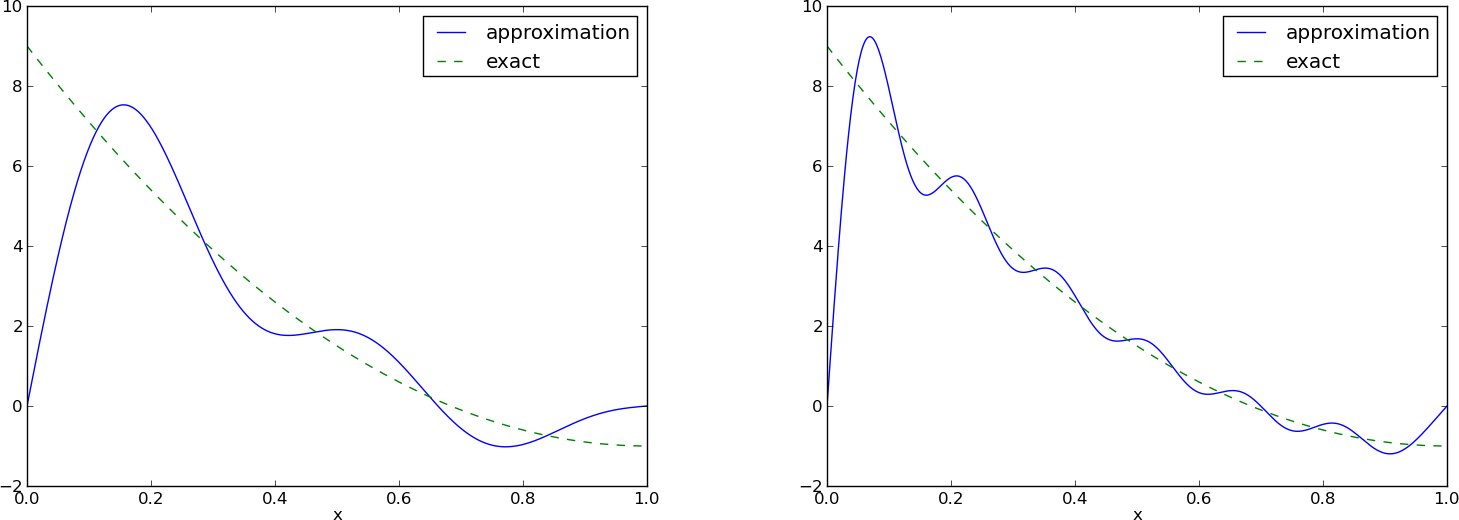 #
#
#
#
# There is an error $f(0)-u(0)=9$ at $x=0$ in [Figure](#fem:approx:global:fig:parabola:sine1) regardless of how large $N$ is, because all ${\psi}_i(0)=0$ and hence
# $u(0)=0$. We may help the approximation to be correct at $x=0$ by
# seeking
#
#
#
# $$
# \begin{equation}
# u(x) = f(0) + \sum_{j\in{\mathcal{I}_s}} c_j{\psi}_j(x)
# {\thinspace .}
# \label{_auto21} \tag{49}
# \end{equation}
# $$
# However, this adjustment introduces a new problem at $x=1$ since
# we now get an error $f(1)-u(1)=f(1)-0=-1$ at this point. A more
# clever adjustment is to replace the $f(0)$ term by a term that
# is $f(0)$ at $x=0$ and $f(1)$ at $x=1$. A simple linear combination
# $f(0)(1-x) + xf(1)$ does the job:
#
#
#
# $$
# \begin{equation}
# u(x) = f(0)(1-x) + xf(1) + \sum_{j\in{\mathcal{I}_s}} c_j{\psi}_j(x)
# {\thinspace .}
# \label{_auto22} \tag{50}
# \end{equation}
# $$
# This adjustment of $u$ alters the linear system slightly. In the general
# case, we set
# $$
# u(x) = B(x) + \sum_{j\in{\mathcal{I}_s}} c_j{\psi}_j(x),
# $$
# and the linear system becomes
# $$
# \sum_{j\in{\mathcal{I}_s}}({\psi}_i,{\psi}_j)c_j = (f-B,{\psi}_i),\quad i\in{\mathcal{I}_s}{\thinspace .}
# $$
# The calculations can still utilize the `least_squares` or
# `least_squares_orth` functions, but solve for $u-b$:
# In[17]:
from src.approx1D import least_squares_orth
f0 = 0; f1 = -1
b = f0*(1-x) + x*f1
u_sum, c = least_squares_orth(f-b, psi, Omega)
u = B + u_sum
# [Figure](#fem:approx:global:fig:parabola:sine2) shows the result
# of the technique for
# ensuring the right boundary values. Even 3 sines can now adjust the
# $f(0)(1-x) + xf(1)$ term such that $u$ approximates the parabola really
# well, at least visually.
#
#
#
#
#
#
#
#
#
#
# There is an error $f(0)-u(0)=9$ at $x=0$ in [Figure](#fem:approx:global:fig:parabola:sine1) regardless of how large $N$ is, because all ${\psi}_i(0)=0$ and hence
# $u(0)=0$. We may help the approximation to be correct at $x=0$ by
# seeking
#
#
#
# $$
# \begin{equation}
# u(x) = f(0) + \sum_{j\in{\mathcal{I}_s}} c_j{\psi}_j(x)
# {\thinspace .}
# \label{_auto21} \tag{49}
# \end{equation}
# $$
# However, this adjustment introduces a new problem at $x=1$ since
# we now get an error $f(1)-u(1)=f(1)-0=-1$ at this point. A more
# clever adjustment is to replace the $f(0)$ term by a term that
# is $f(0)$ at $x=0$ and $f(1)$ at $x=1$. A simple linear combination
# $f(0)(1-x) + xf(1)$ does the job:
#
#
#
# $$
# \begin{equation}
# u(x) = f(0)(1-x) + xf(1) + \sum_{j\in{\mathcal{I}_s}} c_j{\psi}_j(x)
# {\thinspace .}
# \label{_auto22} \tag{50}
# \end{equation}
# $$
# This adjustment of $u$ alters the linear system slightly. In the general
# case, we set
# $$
# u(x) = B(x) + \sum_{j\in{\mathcal{I}_s}} c_j{\psi}_j(x),
# $$
# and the linear system becomes
# $$
# \sum_{j\in{\mathcal{I}_s}}({\psi}_i,{\psi}_j)c_j = (f-B,{\psi}_i),\quad i\in{\mathcal{I}_s}{\thinspace .}
# $$
# The calculations can still utilize the `least_squares` or
# `least_squares_orth` functions, but solve for $u-b$:
# In[17]:
from src.approx1D import least_squares_orth
f0 = 0; f1 = -1
b = f0*(1-x) + x*f1
u_sum, c = least_squares_orth(f-b, psi, Omega)
u = B + u_sum
# [Figure](#fem:approx:global:fig:parabola:sine2) shows the result
# of the technique for
# ensuring the right boundary values. Even 3 sines can now adjust the
# $f(0)(1-x) + xf(1)$ term such that $u$ approximates the parabola really
# well, at least visually.
#
#
#
#
#
# Best approximation of a parabola by a sum of 3 (left) and 11 (right) sine functions with a boundary term.
# #
#
#
#
#
# ## Orthogonal basis functions
#
#
# The choice of sine functions ${\psi}_i(x)=\sin ((i+1)\pi x)$ has a great
# computational advantage: on $\Omega=[0,1]$ these basis functions are
# *orthogonal*, implying that $A_{i,j}=0$ if $i\neq j$. In fact, when
# $V$ contains the basic functions used in a Fourier series expansion,
# the approximation method derived in the section [Approximation principles](#fem:approx:global) results in the classical Fourier series for $f(x)$.
# With orthogonal basis functions we can make the
# `least_squares` function (much) more efficient since we know that
# the matrix is diagonal and only the diagonal elements need to be computed:
# In[18]:
def least_squares_orth(f, psi, Omega):
N = len(psi) - 1
A = [0]*(N+1)
b = [0]*(N+1)
x = sym.Symbol('x')
for i in range(N+1):
A[i] = sym.integrate(psi[i]**2, (x, Omega[0], Omega[1]))
b[i] = sym.integrate(psi[i]*f, (x, Omega[0], Omega[1]))
c = [b[i]/A[i] for i in range(len(b))]
u = 0
for i in range(len(psi)):
u += c[i]*psi[i]
return u, c
# As mentioned in the section [Implementation of the least squares method](#fem:approx:global:LS:code), symbolic integration
# may fail or take a very long time. It is therefore natural to extend the
# implementation above with a version where we can choose between symbolic
# and numerical integration and fall back on the latter if the former
# fails:
# In[19]:
def least_squares_orth(f, psi, Omega, symbolic=True):
N = len(psi) - 1
A = [0]*(N+1) # plain list to hold symbolic expressions
b = [0]*(N+1)
x = sym.Symbol('x')
for i in range(N+1):
# Diagonal matrix term
A[i] = sym.integrate(psi[i]**2, (x, Omega[0], Omega[1]))
# Right-hand side term
integrand = psi[i]*f
if symbolic:
I = sym.integrate(integrand, (x, Omega[0], Omega[1]))
if not symbolic or isinstance(I, sym.Integral):
print(('numerical integration of', integrand))
integrand = sym.lambdify([x], integrand, 'mpmath')
I = mpmath.quad(integrand, [Omega[0], Omega[1]])
b[i] = I
c = [b[i]/A[i] for i in range(len(b))]
u = 0
u = sum(c[i]*psi[i] for i in range(len(psi)))
return u, c
# This function is found in the file [`approx1D.py`](src/approx1D.py). Observe that
# we here assume that
# $\int_\Omega{\varphi}_i^2{\, \mathrm{d}x}$ can always be symbolically computed,
# which is not an unreasonable assumption
# when the basis functions are orthogonal, but there is no guarantee,
# so an improved version of the function above would implement
# numerical integration also for the `A[i,i]` term.
#
# ## Numerical computations
#
# Sometimes the basis functions ${\psi}_i$ and/or the function $f$
# have a nature that makes symbolic integration CPU-time
# consuming or impossible.
# Even though we implemented a fallback on numerical integration
# of $\int f{\varphi}_i {\, \mathrm{d}x}$, considerable time might still be required
# by `sympy` just by *attempting* to integrate symbolically.
# Therefore, it will be handy to have a function for fast
# *numerical integration and numerical solution
# of the linear system*. Below is such a method. It requires
# Python functions `f(x)` and `psi(x,i)` for $f(x)$ and ${\psi}_i(x)$
# as input. The output is a mesh function
# with values `u` on the mesh with points in the array `x`.
# Three numerical integration methods are offered:
# `scipy.integrate.quad` (precision set to $10^{-8}$),
# `mpmath.quad` (about machine precision), and a Trapezoidal
# rule based on the points in `x` (unknown accuracy, but
# increasing with the number of mesh points in `x`).
# In[20]:
def least_squares_numerical(f, psi, N, x,
integration_method='scipy',
orthogonal_basis=False):
import scipy.integrate
A = np.zeros((N+1, N+1))
b = np.zeros(N+1)
Omega = [x[0], x[-1]]
dx = x[1] - x[0] # assume uniform partition
for i in range(N+1):
j_limit = i+1 if orthogonal_basis else N+1
for j in range(i, j_limit):
print(('(%d,%d)' % (i, j)))
if integration_method == 'scipy':
A_ij = scipy.integrate.quad(
lambda x: psi(x,i)*psi(x,j),
Omega[0], Omega[1], epsabs=1E-9, epsrel=1E-9)[0]
elif integration_method == 'sympy':
A_ij = mpmath.quad(
lambda x: psi(x,i)*psi(x,j),
[Omega[0], Omega[1]])
else:
values = psi(x,i)*psi(x,j)
A_ij = trapezoidal(values, dx)
A[i,j] = A[j,i] = A_ij
if integration_method == 'scipy':
b_i = scipy.integrate.quad(
lambda x: f(x)*psi(x,i), Omega[0], Omega[1],
epsabs=1E-9, epsrel=1E-9)[0]
elif integration_method == 'sympy':
b_i = mpmath.quad(
lambda x: f(x)*psi(x,i), [Omega[0], Omega[1]])
else:
values = f(x)*psi(x,i)
b_i = trapezoidal(values, dx)
b[i] = b_i
c = b/np.diag(A) if orthogonal_basis else np.linalg.solve(A, b)
u = sum(c[i]*psi(x, i) for i in range(N+1))
return u, c
def trapezoidal(values, dx):
"""Integrate values by the Trapezoidal rule (mesh size dx)."""
return dx*(np.sum(values) - 0.5*values[0] - 0.5*values[-1])
# Here is an example on calling the function:
# In[22]:
def psi(x, i):
return np.sin((i+1)*x)
x = np.linspace(0, 2*pi, 501)
N = 20
u, c = least_squares_numerical(lambda x: np.tanh(x-np.pi), psi, N, x,
orthogonal_basis=True)
# **Remark.**
# The `scipy.integrate.quad` integrator is usually much faster than
# `mpmath.quad`.
#
# # Interpolation
#
# ## The interpolation (or collocation) principle
#
#
#
# The principle of minimizing the distance between $u$ and $f$ is
# an intuitive way of computing a best approximation $u\in V$ to $f$.
# However, there are other approaches as well.
# One is to demand that $u(x_{i}) = f(x_{i})$ at some selected points
# $x_{i}$, $i\in{\mathcal{I}_s}$:
#
#
#
# $$
# \begin{equation}
# u(x_{i}) = \sum_{j\in{\mathcal{I}_s}} c_j {\psi}_j(x_{i}) = f(x_{i}),
# \quad i\in{\mathcal{I}_s}{\thinspace .} \label{_auto24} \tag{52}
# \end{equation}
# $$
# We recognize that the equation $\sum_j c_j {\psi}_j(x_{i}) = f(x_{i})$
# is actually a linear system with $N+1$ unknown coefficients $\left\{ {c}_j \right\}_{j\in{\mathcal{I}_s}}$:
#
#
#
# $$
# \begin{equation}
# \sum_{j\in{\mathcal{I}_s}} A_{i,j}c_j = b_i,\quad i\in{\mathcal{I}_s},
# \label{_auto25} \tag{53}
# \end{equation}
# $$
# with coefficient matrix and right-hand side vector given by
#
#
#
# $$
# \begin{equation}
# A_{i,j} = {\psi}_j(x_{i}),
# \label{_auto26} \tag{54}
# \end{equation}
# $$
#
#
#
# $$
# \begin{equation}
# b_i = f(x_{i}){\thinspace .} \label{_auto27} \tag{55}
# \end{equation}
# $$
# This time the coefficient matrix is not symmetric because
# ${\psi}_j(x_{i})\neq {\psi}_i(x_{j})$ in general.
# The method is often referred to as an *interpolation method*
# since some point values of $f$ are given ($f(x_{i})$) and we
# fit a continuous function $u$ that goes through the $f(x_{i})$ points.
# In this case the $x_{i}$ points are called *interpolation points*.
# When the same approach is used to approximate differential equations,
# one usually applies the name *collocation method* and
# $x_{i}$ are known as *collocation points*.
#
# Given $f$ as a `sympy` symbolic expression `f`, $\left\{ {{\psi}}_i \right\}_{i\in{\mathcal{I}_s}}$
# as a list `psi`, and a set of points $\left\{ {x}_i \right\}_{i\in{\mathcal{I}_s}}$ as a list or array
# `points`, the following Python function sets up and solves the matrix system
# for the coefficients $\left\{ {c}_i \right\}_{i\in{\mathcal{I}_s}}$:
# In[23]:
def interpolation(f, psi, points):
N = len(psi) - 1
A = sym.zeros(N+1, N+1)
b = sym.zeros(N+1, 1)
psi_sym = psi # save symbolic expression
x = sym.Symbol('x')
psi = [sym.lambdify([x], psi[i], 'mpmath') for i in range(N+1)]
f = sym.lambdify([x], f, 'mpmath')
for i in range(N+1):
for j in range(N+1):
A[i,j] = psi[j](points[i])
b[i,0] = f(points[i])
c = A.LUsolve(b)
# c is a sympy Matrix object, turn to list
c = [sym.simplify(c[i,0]) for i in range(c.shape[0])]
u = sym.simplify(sum(c[i]*psi_sym[i] for i in range(N+1)))
return u, c
# The `interpolation` function is a part of the [`approx1D`](src/approx1D.py)
# module.
#
#
# We found it convenient in the above function to turn the expressions `f` and
# `psi` into ordinary Python functions of `x`, which can be called with
# `float` values in the list `points` when building the matrix and
# the right-hand side. The alternative is to use the `subs` method
# to substitute the `x` variable in an expression by an element from
# the `points` list. The following session illustrates both approaches
# in a simple setting:
# In[24]:
x = sym.Symbol('x')
e = x**2 # symbolic expression involving x
p = 0.5 # a value of x
v = e.subs(x, p) # evaluate e for x=p
v
# In[25]:
type(v)
# In[26]:
e = lambdify([x], e) # make Python function of e
type(e)
function
v = e(p) # evaluate e(x) for x=p
v
# In[27]:
type(v)
# A nice feature of the interpolation or collocation method is that it
# avoids computing integrals. However, one has to decide on the location
# of the $x_{i}$ points. A simple, yet common choice, is to
# distribute them uniformly throughout the unit interval.
#
# ### Example
#
# Let us illustrate the interpolation method by approximating
# our parabola $f(x)=10(x-1)^2-1$ by a linear function on $\Omega=[1,2]$,
# using two collocation points $x_0=1+1/3$ and $x_1=1+2/3$:
# In[28]:
x = sym.Symbol('x')
f = 10*(x-1)**2 - 1
psi = [1, x]
Omega = [1, 2]
points = [1 + sym.Rational(1,3), 1 + sym.Rational(2,3)]
u, c = interpolation(f, psi, points)
comparison_plot(f, u, Omega)
# The resulting linear system becomes
# $$
# \left(\begin{array}{ll}
# 1 & 4/3\\
# 1 & 5/3\\
# \end{array}\right)
# \left(\begin{array}{l}
# c_0\\
# c_1\\
# \end{array}\right)
# =
# \left(\begin{array}{l}
# 1/9\\
# 31/9\\
# \end{array}\right)
# $$
# with solution $c_0=-119/9$ and $c_1=10$.
# [Figure](#fem:approx:global:linear:interp:fig1) (left) shows the resulting
# approximation $u=-119/9 + 10x$.
# We can easily test other interpolation points, say $x_0=1$ and $x_1=2$.
# This changes the line quite significantly, see
# [Figure](#fem:approx:global:linear:interp:fig1) (right).
#
#
#
#
#
#
#
#
#
#
#
# ## Orthogonal basis functions
#
#
# The choice of sine functions ${\psi}_i(x)=\sin ((i+1)\pi x)$ has a great
# computational advantage: on $\Omega=[0,1]$ these basis functions are
# *orthogonal*, implying that $A_{i,j}=0$ if $i\neq j$. In fact, when
# $V$ contains the basic functions used in a Fourier series expansion,
# the approximation method derived in the section [Approximation principles](#fem:approx:global) results in the classical Fourier series for $f(x)$.
# With orthogonal basis functions we can make the
# `least_squares` function (much) more efficient since we know that
# the matrix is diagonal and only the diagonal elements need to be computed:
# In[18]:
def least_squares_orth(f, psi, Omega):
N = len(psi) - 1
A = [0]*(N+1)
b = [0]*(N+1)
x = sym.Symbol('x')
for i in range(N+1):
A[i] = sym.integrate(psi[i]**2, (x, Omega[0], Omega[1]))
b[i] = sym.integrate(psi[i]*f, (x, Omega[0], Omega[1]))
c = [b[i]/A[i] for i in range(len(b))]
u = 0
for i in range(len(psi)):
u += c[i]*psi[i]
return u, c
# As mentioned in the section [Implementation of the least squares method](#fem:approx:global:LS:code), symbolic integration
# may fail or take a very long time. It is therefore natural to extend the
# implementation above with a version where we can choose between symbolic
# and numerical integration and fall back on the latter if the former
# fails:
# In[19]:
def least_squares_orth(f, psi, Omega, symbolic=True):
N = len(psi) - 1
A = [0]*(N+1) # plain list to hold symbolic expressions
b = [0]*(N+1)
x = sym.Symbol('x')
for i in range(N+1):
# Diagonal matrix term
A[i] = sym.integrate(psi[i]**2, (x, Omega[0], Omega[1]))
# Right-hand side term
integrand = psi[i]*f
if symbolic:
I = sym.integrate(integrand, (x, Omega[0], Omega[1]))
if not symbolic or isinstance(I, sym.Integral):
print(('numerical integration of', integrand))
integrand = sym.lambdify([x], integrand, 'mpmath')
I = mpmath.quad(integrand, [Omega[0], Omega[1]])
b[i] = I
c = [b[i]/A[i] for i in range(len(b))]
u = 0
u = sum(c[i]*psi[i] for i in range(len(psi)))
return u, c
# This function is found in the file [`approx1D.py`](src/approx1D.py). Observe that
# we here assume that
# $\int_\Omega{\varphi}_i^2{\, \mathrm{d}x}$ can always be symbolically computed,
# which is not an unreasonable assumption
# when the basis functions are orthogonal, but there is no guarantee,
# so an improved version of the function above would implement
# numerical integration also for the `A[i,i]` term.
#
# ## Numerical computations
#
# Sometimes the basis functions ${\psi}_i$ and/or the function $f$
# have a nature that makes symbolic integration CPU-time
# consuming or impossible.
# Even though we implemented a fallback on numerical integration
# of $\int f{\varphi}_i {\, \mathrm{d}x}$, considerable time might still be required
# by `sympy` just by *attempting* to integrate symbolically.
# Therefore, it will be handy to have a function for fast
# *numerical integration and numerical solution
# of the linear system*. Below is such a method. It requires
# Python functions `f(x)` and `psi(x,i)` for $f(x)$ and ${\psi}_i(x)$
# as input. The output is a mesh function
# with values `u` on the mesh with points in the array `x`.
# Three numerical integration methods are offered:
# `scipy.integrate.quad` (precision set to $10^{-8}$),
# `mpmath.quad` (about machine precision), and a Trapezoidal
# rule based on the points in `x` (unknown accuracy, but
# increasing with the number of mesh points in `x`).
# In[20]:
def least_squares_numerical(f, psi, N, x,
integration_method='scipy',
orthogonal_basis=False):
import scipy.integrate
A = np.zeros((N+1, N+1))
b = np.zeros(N+1)
Omega = [x[0], x[-1]]
dx = x[1] - x[0] # assume uniform partition
for i in range(N+1):
j_limit = i+1 if orthogonal_basis else N+1
for j in range(i, j_limit):
print(('(%d,%d)' % (i, j)))
if integration_method == 'scipy':
A_ij = scipy.integrate.quad(
lambda x: psi(x,i)*psi(x,j),
Omega[0], Omega[1], epsabs=1E-9, epsrel=1E-9)[0]
elif integration_method == 'sympy':
A_ij = mpmath.quad(
lambda x: psi(x,i)*psi(x,j),
[Omega[0], Omega[1]])
else:
values = psi(x,i)*psi(x,j)
A_ij = trapezoidal(values, dx)
A[i,j] = A[j,i] = A_ij
if integration_method == 'scipy':
b_i = scipy.integrate.quad(
lambda x: f(x)*psi(x,i), Omega[0], Omega[1],
epsabs=1E-9, epsrel=1E-9)[0]
elif integration_method == 'sympy':
b_i = mpmath.quad(
lambda x: f(x)*psi(x,i), [Omega[0], Omega[1]])
else:
values = f(x)*psi(x,i)
b_i = trapezoidal(values, dx)
b[i] = b_i
c = b/np.diag(A) if orthogonal_basis else np.linalg.solve(A, b)
u = sum(c[i]*psi(x, i) for i in range(N+1))
return u, c
def trapezoidal(values, dx):
"""Integrate values by the Trapezoidal rule (mesh size dx)."""
return dx*(np.sum(values) - 0.5*values[0] - 0.5*values[-1])
# Here is an example on calling the function:
# In[22]:
def psi(x, i):
return np.sin((i+1)*x)
x = np.linspace(0, 2*pi, 501)
N = 20
u, c = least_squares_numerical(lambda x: np.tanh(x-np.pi), psi, N, x,
orthogonal_basis=True)
# **Remark.**
# The `scipy.integrate.quad` integrator is usually much faster than
# `mpmath.quad`.
#
# # Interpolation
#
# ## The interpolation (or collocation) principle
#
#
#
# The principle of minimizing the distance between $u$ and $f$ is
# an intuitive way of computing a best approximation $u\in V$ to $f$.
# However, there are other approaches as well.
# One is to demand that $u(x_{i}) = f(x_{i})$ at some selected points
# $x_{i}$, $i\in{\mathcal{I}_s}$:
#
#
#
# $$
# \begin{equation}
# u(x_{i}) = \sum_{j\in{\mathcal{I}_s}} c_j {\psi}_j(x_{i}) = f(x_{i}),
# \quad i\in{\mathcal{I}_s}{\thinspace .} \label{_auto24} \tag{52}
# \end{equation}
# $$
# We recognize that the equation $\sum_j c_j {\psi}_j(x_{i}) = f(x_{i})$
# is actually a linear system with $N+1$ unknown coefficients $\left\{ {c}_j \right\}_{j\in{\mathcal{I}_s}}$:
#
#
#
# $$
# \begin{equation}
# \sum_{j\in{\mathcal{I}_s}} A_{i,j}c_j = b_i,\quad i\in{\mathcal{I}_s},
# \label{_auto25} \tag{53}
# \end{equation}
# $$
# with coefficient matrix and right-hand side vector given by
#
#
#
# $$
# \begin{equation}
# A_{i,j} = {\psi}_j(x_{i}),
# \label{_auto26} \tag{54}
# \end{equation}
# $$
#
#
#
# $$
# \begin{equation}
# b_i = f(x_{i}){\thinspace .} \label{_auto27} \tag{55}
# \end{equation}
# $$
# This time the coefficient matrix is not symmetric because
# ${\psi}_j(x_{i})\neq {\psi}_i(x_{j})$ in general.
# The method is often referred to as an *interpolation method*
# since some point values of $f$ are given ($f(x_{i})$) and we
# fit a continuous function $u$ that goes through the $f(x_{i})$ points.
# In this case the $x_{i}$ points are called *interpolation points*.
# When the same approach is used to approximate differential equations,
# one usually applies the name *collocation method* and
# $x_{i}$ are known as *collocation points*.
#
# Given $f$ as a `sympy` symbolic expression `f`, $\left\{ {{\psi}}_i \right\}_{i\in{\mathcal{I}_s}}$
# as a list `psi`, and a set of points $\left\{ {x}_i \right\}_{i\in{\mathcal{I}_s}}$ as a list or array
# `points`, the following Python function sets up and solves the matrix system
# for the coefficients $\left\{ {c}_i \right\}_{i\in{\mathcal{I}_s}}$:
# In[23]:
def interpolation(f, psi, points):
N = len(psi) - 1
A = sym.zeros(N+1, N+1)
b = sym.zeros(N+1, 1)
psi_sym = psi # save symbolic expression
x = sym.Symbol('x')
psi = [sym.lambdify([x], psi[i], 'mpmath') for i in range(N+1)]
f = sym.lambdify([x], f, 'mpmath')
for i in range(N+1):
for j in range(N+1):
A[i,j] = psi[j](points[i])
b[i,0] = f(points[i])
c = A.LUsolve(b)
# c is a sympy Matrix object, turn to list
c = [sym.simplify(c[i,0]) for i in range(c.shape[0])]
u = sym.simplify(sum(c[i]*psi_sym[i] for i in range(N+1)))
return u, c
# The `interpolation` function is a part of the [`approx1D`](src/approx1D.py)
# module.
#
#
# We found it convenient in the above function to turn the expressions `f` and
# `psi` into ordinary Python functions of `x`, which can be called with
# `float` values in the list `points` when building the matrix and
# the right-hand side. The alternative is to use the `subs` method
# to substitute the `x` variable in an expression by an element from
# the `points` list. The following session illustrates both approaches
# in a simple setting:
# In[24]:
x = sym.Symbol('x')
e = x**2 # symbolic expression involving x
p = 0.5 # a value of x
v = e.subs(x, p) # evaluate e for x=p
v
# In[25]:
type(v)
# In[26]:
e = lambdify([x], e) # make Python function of e
type(e)
function
v = e(p) # evaluate e(x) for x=p
v
# In[27]:
type(v)
# A nice feature of the interpolation or collocation method is that it
# avoids computing integrals. However, one has to decide on the location
# of the $x_{i}$ points. A simple, yet common choice, is to
# distribute them uniformly throughout the unit interval.
#
# ### Example
#
# Let us illustrate the interpolation method by approximating
# our parabola $f(x)=10(x-1)^2-1$ by a linear function on $\Omega=[1,2]$,
# using two collocation points $x_0=1+1/3$ and $x_1=1+2/3$:
# In[28]:
x = sym.Symbol('x')
f = 10*(x-1)**2 - 1
psi = [1, x]
Omega = [1, 2]
points = [1 + sym.Rational(1,3), 1 + sym.Rational(2,3)]
u, c = interpolation(f, psi, points)
comparison_plot(f, u, Omega)
# The resulting linear system becomes
# $$
# \left(\begin{array}{ll}
# 1 & 4/3\\
# 1 & 5/3\\
# \end{array}\right)
# \left(\begin{array}{l}
# c_0\\
# c_1\\
# \end{array}\right)
# =
# \left(\begin{array}{l}
# 1/9\\
# 31/9\\
# \end{array}\right)
# $$
# with solution $c_0=-119/9$ and $c_1=10$.
# [Figure](#fem:approx:global:linear:interp:fig1) (left) shows the resulting
# approximation $u=-119/9 + 10x$.
# We can easily test other interpolation points, say $x_0=1$ and $x_1=2$.
# This changes the line quite significantly, see
# [Figure](#fem:approx:global:linear:interp:fig1) (right).
#
#
#
#
#
# Approximation of a parabola by linear functions computed by two interpolation points: 4/3 and 5/3 (left) versus 1 and 2 (right).
# #
#
#
#
# ## Lagrange polynomials
#
#
# In the section [Fourier series](#fem:approx:global:Fourier) we explained the advantage
# of having a diagonal matrix: formulas for the coefficients
# $\left\{ {c}_i \right\}_{i\in{\mathcal{I}_s}}$ can then be derived by hand. For an interpolation (or
# collocation) method a diagonal matrix implies that ${\psi}_j(x_{i})
# = 0$ if $i\neq j$. One set of basis functions ${\psi}_i(x)$ with this
# property is the *Lagrange interpolating polynomials*, or just
# *Lagrange polynomials*. (Although the functions are named after
# Lagrange, they were first discovered by Waring in 1779, rediscovered
# by Euler in 1783, and published by Lagrange in 1795.) Lagrange
# polynomials are key building blocks in the finite element method, so
# familiarity with these polynomials will be required anyway.
#
# A Lagrange polynomial can be written as
#
#
#
# $$
# \begin{equation}
# {\psi}_i(x) =
# \prod_{j=0,j\neq i}^N
# \frac{x-x_{j}}{x_{i}-x_{j}}
# = \frac{x-x_0}{x_{i}-x_0}\cdots\frac{x-x_{i-1}}{x_{i}-x_{i-1}}\frac{x-x_{i+1}}{x_{i}-x_{i+1}}
# \cdots\frac{x-x_N}{x_{i}-x_N},
# \label{fem:approx:global:Lagrange:poly} \tag{56}
# \end{equation}
# $$
# for $i\in{\mathcal{I}_s}$.
# We see from ([56](#fem:approx:global:Lagrange:poly)) that all the ${\psi}_i$
# functions are polynomials of degree $N$ which have the property
#
#
#
# $$
# \begin{equation}
# {\psi}_i(x_s) = \delta_{is},\quad \delta_{is} =
# \left\lbrace\begin{array}{ll}
# 1, & i=s,\\
# 0, & i\neq s,
# \end{array}\right.
# \label{fem:inter:prop} \tag{57}
# \end{equation}
# $$
# when $x_s$ is an interpolation (collocation) point.
# Here we have used the *Kronecker delta* symbol $\delta_{is}$.
# This property implies that $A$ is a diagonal matrix, i.e., $A_{i,j}=0$ for $i\neq j$ and
# $A_{i,j}=1$ when $i=j$. The solution of the linear system is
# then simply
#
#
#
# $$
# \begin{equation}
# c_i = f(x_{i}),\quad i\in{\mathcal{I}_s},
# \label{_auto28} \tag{58}
# \end{equation}
# $$
# and
#
#
#
# $$
# \begin{equation}
# u(x) = \sum_{j\in{\mathcal{I}_s}} c_i {\psi}_i(x) = \sum_{j\in{\mathcal{I}_s}} f(x_{i}){\psi}_i(x){\thinspace .} \label{_auto29} \tag{59}
# \end{equation}
# $$
# We remark however that ([57](#fem:inter:prop)) does not necessarily imply that the matrix
# obtained by the least squares or projection methods is diagonal.
#
#
# The following function computes the Lagrange interpolating polynomial
# ${\psi}_i(x)$ on the unit interval (0,1), given the interpolation points $x_{0},\ldots,x_{N}$ in
# the list or array `points`:
# In[29]:
def Lagrange_polynomial(x, i, points):
p = 1
for k in range(len(points)):
if k != i:
p *= (x - points[k])/(points[i] - points[k])
return p
# The next function computes a complete basis, ${\psi}_0,\ldots,{\psi}_N$, using equidistant points throughout
# $\Omega$:
# In[30]:
def Lagrange_polynomials_01(x, N):
if isinstance(x, sym.Symbol):
h = sym.Rational(1, N-1)
else:
h = 1.0/(N-1)
points = [i*h for i in range(N)]
psi = [Lagrange_polynomial(x, i, points) for i in range(N)]
return psi, points
# When `x` is a `sym.Symbol` object, we let the spacing between the
# interpolation points, `h`, be a `sympy` rational number, so that we
# get nice end results in the formulas for ${\psi}_i$. The other case,
# when `x` is a plain Python `float`, signifies numerical computing, and
# then we let `h` be a floating-point number. Observe that the
# `Lagrange_polynomial` function works equally well in the symbolic and
# numerical case - just think of `x` being a `sym.Symbol` object or a
# Python `float`. A little interactive session illustrates the
# difference between symbolic and numerical computing of the basis
# functions and points:
# In[31]:
x = sym.Symbol('x')
psi, points = Lagrange_polynomials_01(x, N=2)
points
# In[32]:
psi
# In[33]:
x = 0.5 # numerical computing
psi, points = Lagrange_polynomials_01(x, N=2)
points
# In[34]:
psi
# That is, when used symbolically, the `Lagrange_polynomials_01`
# function returns the symbolic expression for the Lagrange functions
# while when `x` is a numerical value the function returns the value of
# the basis function evaluate in `x`. In the present example only the
# second basis function should be 1 in the mid-point while the others
# are zero according to ([57](#fem:inter:prop)).
#
#
# ### Approximation of a polynomial
#
# The Galerkin or least squares methods lead to an exact approximation
# if $f$ lies in the space spanned by the basis functions. It could be
# of interest to see how the interpolation method with Lagrange
# polynomials as the basis is able to approximate a polynomial, e.g., a
# parabola. Running
# In[37]:
x = sym.Symbol('x')
for N in 2, 4, 5, 6, 8, 10, 12:
f = x**2
psi, points = Lagrange_polynomials_01(x, N)
u = interpolation(f, psi, points)
# shows the result that up to `N=4` we achieve an exact approximation,
# and then round-off errors start to grow, such that
# `N=15` leads to a 15-degree polynomial for $u$ where
# the coefficients in front of $x^r$ for $r>2$ are
# of size $10^{-5}$ and smaller. As the matrix is ill-conditioned
# and we use floating-point arithmetic, we do not obtain the exact
# solution. Still, we get a solution that is visually identical to the
# exact solution. The reason is that the ill-conditioning causes
# the system to have many solutions very close to the true solution.
# While we are lucky for `N=15` and obtain a solution that is
# visually identical to the true solution, ill-conditioning may also
# result in completely wrong results. As we continue with higher values, `N=20` reveals that the
# procedure is starting to fall apart as the approximate solution is around 0.9 at $x=1.0$,
# where it should have
# been $1.0$. At `N=30` the approximate solution is around $5\cdot10^8 $ at $x=1$.
#
#
# ### Successful example
#
# Trying out the Lagrange polynomial basis for approximating
# $f(x)=\sin 2\pi x$ on $\Omega =[0,1]$ with the least squares
# and the interpolation techniques can be done by
# In[36]:
x = sym.Symbol('x')
f = sym.sin(2*sym.pi*x)
psi, points = Lagrange_polynomials_01(x, N)
Omega=[0, 1]
u, c = least_squares(f, psi, Omega)
comparison_plot(f, u, Omega)
u, c = interpolation(f, psi, points)
comparison_plot(f, u, Omega)
# [Figure](#fem:approx:global:Lagrange:fig:sine:ls:colloc) shows the results.
# There is a difference between the least squares and the interpolation
# technique but the difference decreases rapidly with increasing $N$.
#
#
#
#
#
#
#
#
#
#
# ## Lagrange polynomials
#
#
# In the section [Fourier series](#fem:approx:global:Fourier) we explained the advantage
# of having a diagonal matrix: formulas for the coefficients
# $\left\{ {c}_i \right\}_{i\in{\mathcal{I}_s}}$ can then be derived by hand. For an interpolation (or
# collocation) method a diagonal matrix implies that ${\psi}_j(x_{i})
# = 0$ if $i\neq j$. One set of basis functions ${\psi}_i(x)$ with this
# property is the *Lagrange interpolating polynomials*, or just
# *Lagrange polynomials*. (Although the functions are named after
# Lagrange, they were first discovered by Waring in 1779, rediscovered
# by Euler in 1783, and published by Lagrange in 1795.) Lagrange
# polynomials are key building blocks in the finite element method, so
# familiarity with these polynomials will be required anyway.
#
# A Lagrange polynomial can be written as
#
#
#
# $$
# \begin{equation}
# {\psi}_i(x) =
# \prod_{j=0,j\neq i}^N
# \frac{x-x_{j}}{x_{i}-x_{j}}
# = \frac{x-x_0}{x_{i}-x_0}\cdots\frac{x-x_{i-1}}{x_{i}-x_{i-1}}\frac{x-x_{i+1}}{x_{i}-x_{i+1}}
# \cdots\frac{x-x_N}{x_{i}-x_N},
# \label{fem:approx:global:Lagrange:poly} \tag{56}
# \end{equation}
# $$
# for $i\in{\mathcal{I}_s}$.
# We see from ([56](#fem:approx:global:Lagrange:poly)) that all the ${\psi}_i$
# functions are polynomials of degree $N$ which have the property
#
#
#
# $$
# \begin{equation}
# {\psi}_i(x_s) = \delta_{is},\quad \delta_{is} =
# \left\lbrace\begin{array}{ll}
# 1, & i=s,\\
# 0, & i\neq s,
# \end{array}\right.
# \label{fem:inter:prop} \tag{57}
# \end{equation}
# $$
# when $x_s$ is an interpolation (collocation) point.
# Here we have used the *Kronecker delta* symbol $\delta_{is}$.
# This property implies that $A$ is a diagonal matrix, i.e., $A_{i,j}=0$ for $i\neq j$ and
# $A_{i,j}=1$ when $i=j$. The solution of the linear system is
# then simply
#
#
#
# $$
# \begin{equation}
# c_i = f(x_{i}),\quad i\in{\mathcal{I}_s},
# \label{_auto28} \tag{58}
# \end{equation}
# $$
# and
#
#
#
# $$
# \begin{equation}
# u(x) = \sum_{j\in{\mathcal{I}_s}} c_i {\psi}_i(x) = \sum_{j\in{\mathcal{I}_s}} f(x_{i}){\psi}_i(x){\thinspace .} \label{_auto29} \tag{59}
# \end{equation}
# $$
# We remark however that ([57](#fem:inter:prop)) does not necessarily imply that the matrix
# obtained by the least squares or projection methods is diagonal.
#
#
# The following function computes the Lagrange interpolating polynomial
# ${\psi}_i(x)$ on the unit interval (0,1), given the interpolation points $x_{0},\ldots,x_{N}$ in
# the list or array `points`:
# In[29]:
def Lagrange_polynomial(x, i, points):
p = 1
for k in range(len(points)):
if k != i:
p *= (x - points[k])/(points[i] - points[k])
return p
# The next function computes a complete basis, ${\psi}_0,\ldots,{\psi}_N$, using equidistant points throughout
# $\Omega$:
# In[30]:
def Lagrange_polynomials_01(x, N):
if isinstance(x, sym.Symbol):
h = sym.Rational(1, N-1)
else:
h = 1.0/(N-1)
points = [i*h for i in range(N)]
psi = [Lagrange_polynomial(x, i, points) for i in range(N)]
return psi, points
# When `x` is a `sym.Symbol` object, we let the spacing between the
# interpolation points, `h`, be a `sympy` rational number, so that we
# get nice end results in the formulas for ${\psi}_i$. The other case,
# when `x` is a plain Python `float`, signifies numerical computing, and
# then we let `h` be a floating-point number. Observe that the
# `Lagrange_polynomial` function works equally well in the symbolic and
# numerical case - just think of `x` being a `sym.Symbol` object or a
# Python `float`. A little interactive session illustrates the
# difference between symbolic and numerical computing of the basis
# functions and points:
# In[31]:
x = sym.Symbol('x')
psi, points = Lagrange_polynomials_01(x, N=2)
points
# In[32]:
psi
# In[33]:
x = 0.5 # numerical computing
psi, points = Lagrange_polynomials_01(x, N=2)
points
# In[34]:
psi
# That is, when used symbolically, the `Lagrange_polynomials_01`
# function returns the symbolic expression for the Lagrange functions
# while when `x` is a numerical value the function returns the value of
# the basis function evaluate in `x`. In the present example only the
# second basis function should be 1 in the mid-point while the others
# are zero according to ([57](#fem:inter:prop)).
#
#
# ### Approximation of a polynomial
#
# The Galerkin or least squares methods lead to an exact approximation
# if $f$ lies in the space spanned by the basis functions. It could be
# of interest to see how the interpolation method with Lagrange
# polynomials as the basis is able to approximate a polynomial, e.g., a
# parabola. Running
# In[37]:
x = sym.Symbol('x')
for N in 2, 4, 5, 6, 8, 10, 12:
f = x**2
psi, points = Lagrange_polynomials_01(x, N)
u = interpolation(f, psi, points)
# shows the result that up to `N=4` we achieve an exact approximation,
# and then round-off errors start to grow, such that
# `N=15` leads to a 15-degree polynomial for $u$ where
# the coefficients in front of $x^r$ for $r>2$ are
# of size $10^{-5}$ and smaller. As the matrix is ill-conditioned
# and we use floating-point arithmetic, we do not obtain the exact
# solution. Still, we get a solution that is visually identical to the
# exact solution. The reason is that the ill-conditioning causes
# the system to have many solutions very close to the true solution.
# While we are lucky for `N=15` and obtain a solution that is
# visually identical to the true solution, ill-conditioning may also
# result in completely wrong results. As we continue with higher values, `N=20` reveals that the
# procedure is starting to fall apart as the approximate solution is around 0.9 at $x=1.0$,
# where it should have
# been $1.0$. At `N=30` the approximate solution is around $5\cdot10^8 $ at $x=1$.
#
#
# ### Successful example
#
# Trying out the Lagrange polynomial basis for approximating
# $f(x)=\sin 2\pi x$ on $\Omega =[0,1]$ with the least squares
# and the interpolation techniques can be done by
# In[36]:
x = sym.Symbol('x')
f = sym.sin(2*sym.pi*x)
psi, points = Lagrange_polynomials_01(x, N)
Omega=[0, 1]
u, c = least_squares(f, psi, Omega)
comparison_plot(f, u, Omega)
u, c = interpolation(f, psi, points)
comparison_plot(f, u, Omega)
# [Figure](#fem:approx:global:Lagrange:fig:sine:ls:colloc) shows the results.
# There is a difference between the least squares and the interpolation
# technique but the difference decreases rapidly with increasing $N$.
#
#
#
#
#
# Approximation via least squares (left) and interpolation (right) of a sine function by Lagrange interpolating polynomials of degree 3.
# #
#
#
#
#
# ### Less successful example
#
# The next example concerns interpolating $f(x)=|1-2x|$ on $\Omega
# =[0,1]$ using Lagrange polynomials. [Figure](#fem:approx:global:Lagrange:fig:abs:Lag:unif:7:14) shows a peculiar
# effect: the approximation starts to oscillate more and more as $N$
# grows. This numerical artifact is not surprising when looking at the
# individual Lagrange polynomials. [Figure](#fem:approx:global:Lagrange:fig:abs:Lag:unif:osc) shows two such
# polynomials, $\psi_2(x)$ and $\psi_7(x)$, both of degree 11 and
# computed from uniformly spaced points $x_{i}=i/11$,
# $i=0,\ldots,11$, marked with circles. We clearly see the property of
# Lagrange polynomials: $\psi_2(x_{i})=0$ and $\psi_7(x_{i})=0$ for
# all $i$, except $\psi_2(x_{2})=1$ and $\psi_7(x_{7})=1$. The most
# striking feature, however, is the dominating oscillation near the
# boundary where $\psi_2>5$ and $\psi_7=-10$ in some points. The reason is easy to understand: since we force the
# functions to be zero at so many points, a polynomial of high degree is
# forced to oscillate between the points. This is called
# *Runge's phenomenon* and you can read a more detailed explanation on
# [Wikipedia](http://en.wikipedia.org/wiki/Runge%27s_phenomenon).
#
#
# ### Remedy for strong oscillations
#
# The oscillations can be reduced by a more clever choice of
# interpolation points, called the *Chebyshev nodes*:
#
#
#
# $$
# \begin{equation}
# x_{i} = \frac{1}{2} (a+b) + \frac{1}{2}(b-a)\cos\left( \frac{2i+1}{2(N+1)}pi\right),\quad i=0\ldots,N,
# \label{_auto30} \tag{60}
# \end{equation}
# $$
# on the interval $\Omega = [a,b]$.
# Here is a flexible version of the `Lagrange_polynomials_01` function above,
# valid for any interval $\Omega =[a,b]$ and with the possibility to generate
# both uniformly distributed points and Chebyshev nodes:
# In[39]:
def Lagrange_polynomials(x, N, Omega, point_distribution='uniform'):
if point_distribution == 'uniform':
if isinstance(x, sym.Symbol):
h = sym.Rational(Omega[1] - Omega[0], N)
else:
h = (Omega[1] - Omega[0])/float(N)
points = [Omega[0] + i*h for i in range(N+1)]
elif point_distribution == 'Chebyshev':
points = Chebyshev_nodes(Omega[0], Omega[1], N)
psi = [Lagrange_polynomial(x, i, points) for i in range(N+1)]
return psi, points
def Chebyshev_nodes(a, b, N):
from math import cos, pi
return [0.5*(a+b) + 0.5*(b-a)*cos(float(2*i+1)/(2*(N+1))*pi) \
for i in range(N+1)]
# All the functions computing Lagrange polynomials listed
# above are found in the module file `Lagrange.py`.
#
# [Figure](#fem:approx:global:Lagrange:fig:abs:Lag:Cheb:7:14) shows the
# improvement of using Chebyshev nodes, compared with the equidistant
# points in [Figure](#fem:approx:global:Lagrange:fig:abs:Lag:unif:7:14). The reason for
# this improvement is that the corresponding Lagrange polynomials have
# much smaller oscillations, which can be seen by comparing [Figure](#fem:approx:global:Lagrange:fig:abs:Lag:Cheb:osc) (Chebyshev
# points) with [Figure](#fem:approx:global:Lagrange:fig:abs:Lag:unif:osc) (equidistant
# points). Note the different scale on the vertical axes in the two
# figures and also that the Chebyshev points tend to cluster
# more around the element boundaries.
#
#
# Another cure for undesired oscillations of higher-degree interpolating
# polynomials is to use lower-degree Lagrange polynomials on many small
# patches of the domain. This is actually the idea pursued in the finite
# element method. For instance, linear Lagrange polynomials on $[0,1/2]$
# and $[1/2,1]$ would yield a perfect approximation to $f(x)=|1-2x|$ on
# $\Omega = [0,1]$ since $f$ is piecewise linear.
#
#
#
#
#
#
#
#
#
#
#
# ### Less successful example
#
# The next example concerns interpolating $f(x)=|1-2x|$ on $\Omega
# =[0,1]$ using Lagrange polynomials. [Figure](#fem:approx:global:Lagrange:fig:abs:Lag:unif:7:14) shows a peculiar
# effect: the approximation starts to oscillate more and more as $N$
# grows. This numerical artifact is not surprising when looking at the
# individual Lagrange polynomials. [Figure](#fem:approx:global:Lagrange:fig:abs:Lag:unif:osc) shows two such
# polynomials, $\psi_2(x)$ and $\psi_7(x)$, both of degree 11 and
# computed from uniformly spaced points $x_{i}=i/11$,
# $i=0,\ldots,11$, marked with circles. We clearly see the property of
# Lagrange polynomials: $\psi_2(x_{i})=0$ and $\psi_7(x_{i})=0$ for
# all $i$, except $\psi_2(x_{2})=1$ and $\psi_7(x_{7})=1$. The most
# striking feature, however, is the dominating oscillation near the
# boundary where $\psi_2>5$ and $\psi_7=-10$ in some points. The reason is easy to understand: since we force the
# functions to be zero at so many points, a polynomial of high degree is
# forced to oscillate between the points. This is called
# *Runge's phenomenon* and you can read a more detailed explanation on
# [Wikipedia](http://en.wikipedia.org/wiki/Runge%27s_phenomenon).
#
#
# ### Remedy for strong oscillations
#
# The oscillations can be reduced by a more clever choice of
# interpolation points, called the *Chebyshev nodes*:
#
#
#
# $$
# \begin{equation}
# x_{i} = \frac{1}{2} (a+b) + \frac{1}{2}(b-a)\cos\left( \frac{2i+1}{2(N+1)}pi\right),\quad i=0\ldots,N,
# \label{_auto30} \tag{60}
# \end{equation}
# $$
# on the interval $\Omega = [a,b]$.
# Here is a flexible version of the `Lagrange_polynomials_01` function above,
# valid for any interval $\Omega =[a,b]$ and with the possibility to generate
# both uniformly distributed points and Chebyshev nodes:
# In[39]:
def Lagrange_polynomials(x, N, Omega, point_distribution='uniform'):
if point_distribution == 'uniform':
if isinstance(x, sym.Symbol):
h = sym.Rational(Omega[1] - Omega[0], N)
else:
h = (Omega[1] - Omega[0])/float(N)
points = [Omega[0] + i*h for i in range(N+1)]
elif point_distribution == 'Chebyshev':
points = Chebyshev_nodes(Omega[0], Omega[1], N)
psi = [Lagrange_polynomial(x, i, points) for i in range(N+1)]
return psi, points
def Chebyshev_nodes(a, b, N):
from math import cos, pi
return [0.5*(a+b) + 0.5*(b-a)*cos(float(2*i+1)/(2*(N+1))*pi) \
for i in range(N+1)]
# All the functions computing Lagrange polynomials listed
# above are found in the module file `Lagrange.py`.
#
# [Figure](#fem:approx:global:Lagrange:fig:abs:Lag:Cheb:7:14) shows the
# improvement of using Chebyshev nodes, compared with the equidistant
# points in [Figure](#fem:approx:global:Lagrange:fig:abs:Lag:unif:7:14). The reason for
# this improvement is that the corresponding Lagrange polynomials have
# much smaller oscillations, which can be seen by comparing [Figure](#fem:approx:global:Lagrange:fig:abs:Lag:Cheb:osc) (Chebyshev
# points) with [Figure](#fem:approx:global:Lagrange:fig:abs:Lag:unif:osc) (equidistant
# points). Note the different scale on the vertical axes in the two
# figures and also that the Chebyshev points tend to cluster
# more around the element boundaries.
#
#
# Another cure for undesired oscillations of higher-degree interpolating
# polynomials is to use lower-degree Lagrange polynomials on many small
# patches of the domain. This is actually the idea pursued in the finite
# element method. For instance, linear Lagrange polynomials on $[0,1/2]$
# and $[1/2,1]$ would yield a perfect approximation to $f(x)=|1-2x|$ on
# $\Omega = [0,1]$ since $f$ is piecewise linear.
#
#
#
#
#
# Interpolation of an absolute value function by Lagrange polynomials and uniformly distributed interpolation points: degree 7 (left) and 14 (right).
# #
#
#
#
#
#
#
#
#
#
#
#
#
#
#
#
#
# Illustration of the oscillatory behavior of two Lagrange polynomials based on 12 uniformly spaced points (marked by circles).
# #
#
#
#
#
#
#
#
#
#
#
#
#
#
#
#
#
#
#
# Interpolation of an absolute value function by Lagrange polynomials and Chebyshev nodes as interpolation points: degree 7 (left) and 14 (right).
# #
#
#
#
#
#
#
#
#
#
#
#
#
#
#
#
#
# Illustration of the less oscillatory behavior of two Lagrange polynomials based on 12 Chebyshev points (marked by circles). Note that the y-axis is different from [Figure](#fem:approx:global:Lagrange:fig:abs:Lag:unif:osc).
#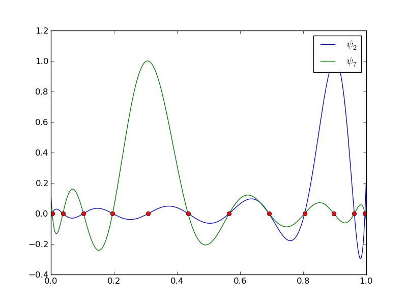 #
#
#
#
# How does the least squares or projection methods work with Lagrange
# polynomials?
# We can just call the `least_squares` function, but
# `sympy` has problems integrating the $f(x)=|1-2x|$
# function times a polynomial, so we need to fall back on numerical
# integration.
# In[40]:
def least_squares(f, psi, Omega):
N = len(psi) - 1
A = sym.zeros(N+1, N+1)
b = sym.zeros(N+1, 1)
x = sym.Symbol('x')
for i in range(N+1):
for j in range(i, N+1):
integrand = psi[i]*psi[j]
I = sym.integrate(integrand, (x, Omega[0], Omega[1]))
if isinstance(I, sym.Integral):
# Could not integrate symbolically, fall back
# on numerical integration with mpmath.quad
integrand = sym.lambdify([x], integrand, 'mpmath')
I = mpmath.quad(integrand, [Omega[0], Omega[1]])
A[i,j] = A[j,i] = I
integrand = psi[i]*f
I = sym.integrate(integrand, (x, Omega[0], Omega[1]))
if isinstance(I, sym.Integral):
integrand = sym.lambdify([x], integrand, 'mpmath')
I = mpmath.quad(integrand, [Omega[0], Omega[1]])
b[i,0] = I
c = A.LUsolve(b)
c = [sym.simplify(c[i,0]) for i in range(c.shape[0])]
u = sum(c[i]*psi[i] for i in range(len(psi)))
return u, c
#
#
#
#
#
#
#
#
#
#
#
#
#
#
# How does the least squares or projection methods work with Lagrange
# polynomials?
# We can just call the `least_squares` function, but
# `sympy` has problems integrating the $f(x)=|1-2x|$
# function times a polynomial, so we need to fall back on numerical
# integration.
# In[40]:
def least_squares(f, psi, Omega):
N = len(psi) - 1
A = sym.zeros(N+1, N+1)
b = sym.zeros(N+1, 1)
x = sym.Symbol('x')
for i in range(N+1):
for j in range(i, N+1):
integrand = psi[i]*psi[j]
I = sym.integrate(integrand, (x, Omega[0], Omega[1]))
if isinstance(I, sym.Integral):
# Could not integrate symbolically, fall back
# on numerical integration with mpmath.quad
integrand = sym.lambdify([x], integrand, 'mpmath')
I = mpmath.quad(integrand, [Omega[0], Omega[1]])
A[i,j] = A[j,i] = I
integrand = psi[i]*f
I = sym.integrate(integrand, (x, Omega[0], Omega[1]))
if isinstance(I, sym.Integral):
integrand = sym.lambdify([x], integrand, 'mpmath')
I = mpmath.quad(integrand, [Omega[0], Omega[1]])
b[i,0] = I
c = A.LUsolve(b)
c = [sym.simplify(c[i,0]) for i in range(c.shape[0])]
u = sum(c[i]*psi[i] for i in range(len(psi)))
return u, c
#
#
#
#
#
#
#
#
#
# Illustration of an approximation of the absolute value function using the least square method .
# #
#
#
#
#
#
#
# ## Bernstein polynomials
#
#
# An alternative to the Taylor and Lagrange families of polynomials
# are the Bernstein polynomials.
# These polynomials are popular in visualization and we include a
# presentation of them for completeness. Furthermore, as we
# will demonstrate, the choice of basis functions may matter
# in terms of accuracy and efficiency.
# In fact, in finite element methods,
# a main challenge, from a numerical analysis point of view,
# is to determine appropriate basis functions for
# a particular purpose or equation.
#
# On the unit interval, the Bernstein
# polynomials are defined in terms of powers of $x$ and $1-x$
# (the barycentric coordinates of the unit interval) as
#
#
#
# $$
# \begin{equation}
# B_{i,n} = \binom{n}{i} x^i (1-x)^{n-i}, \quad i=0, \ldots, n .
# \label{bernstein:basis} \tag{61}
# \end{equation}
# $$
#
#
#
#
#
#
#
#
#
#
#
#
# ## Bernstein polynomials
#
#
# An alternative to the Taylor and Lagrange families of polynomials
# are the Bernstein polynomials.
# These polynomials are popular in visualization and we include a
# presentation of them for completeness. Furthermore, as we
# will demonstrate, the choice of basis functions may matter
# in terms of accuracy and efficiency.
# In fact, in finite element methods,
# a main challenge, from a numerical analysis point of view,
# is to determine appropriate basis functions for
# a particular purpose or equation.
#
# On the unit interval, the Bernstein
# polynomials are defined in terms of powers of $x$ and $1-x$
# (the barycentric coordinates of the unit interval) as
#
#
#
# $$
# \begin{equation}
# B_{i,n} = \binom{n}{i} x^i (1-x)^{n-i}, \quad i=0, \ldots, n .
# \label{bernstein:basis} \tag{61}
# \end{equation}
# $$
#
#
#
#
# The nine functions of a Bernstein basis of order 8.
# #
#
#
#
#
#
#
#
#
#
#
#
#
#
#
#
#
# The nine functions of a Lagrange basis of order 8.
# #
#
#
#
#
#
# The [Figure](#Bernstein_basis_8) shows the basis functions of a Bernstein basis of order 8.
# This figure should be compared against [Figure](#Lagrange_basis_8), which
# shows the corresponding Lagrange basis of order 8.
# The Lagrange basis is convenient because it is a nodal basis, that is; the basis functions are 1 in their nodal points and zero at all other nodal points as described by ([57](#fem:inter:prop)).
# However, looking at [Figure](#Lagrange_basis_8)
# we also notice that the basis function are oscillatory and have absolute
# values that are significantly larger than 1 between the nodal points.
# Consider for instance the basis function represented by the purple color.
# It is 1 at $x=0.5$ and 0 at all other nodal points
# and hence this basis function represents the value at the mid-point.
# However, this function also has strong
# negative contributions close to the element boundaries where
# it takes negative values lower than $-2$.
# For the Bernstein basis, all functions are positive and
# all functions output values in $[0,1]$. Therefore there is no oscillatory behavior.
# The main disadvantage of the Bernstein basis is that the basis is not
# a nodal basis. In fact, all functions contribute everywhere except $x=0$ and $x=1$.
#
# **Notice.**
#
# We have considered approximation with a sinusoidal basis and with Lagrange or Bernstein polynomials,
# all of which are frequently used for scientific computing. The Lagrange polynomials (of various
# order) are extensively used in finite element methods, while the Bernstein polynomials are more used
# in computational geometry. The Lagrange and the Bernstein families are, however, but a few in the jungle of polynomial
# spaces used for finite element computations and their efficiency and accuracy can vary quite substantially.
# Furthermore, while a method may be efficient and accurate for one type of PDE it might not even converge for
# another type of PDE. The development and analysis of finite element methods for different purposes is currently an intense research field
# and has been so for several decades.
# FEniCS has implemented a wide range of polynomial spaces and has a general
# framework for implementing new elements. While finite element methods
# explore different families of polynomials, the so-called spectral methods explore the use
# of sinusoidal functions or polynomials with high order. From an abstract point of view, the different methods
# can all be obtained simply by changing the basis for the trial and test functions. However, their
# efficiency and accuracy may vary substantially.
# # Approximation of functions in higher dimensions
#
#
# All the concepts and algorithms developed for approximation of 1D functions
# $f(x)$ can readily be extended to 2D functions $f(x,y)$ and 3D functions
# $f(x,y,z)$. Basically, the extensions consist of defining basis functions
# ${\psi}_i(x,y)$ or ${\psi}_i(x,y,z)$ over some domain $\Omega$, and
# for the least squares and Galerkin methods, the integration is done over
# $\Omega$.
#
# As in 1D, the least squares and projection/Galerkin methods
# lead to linear systems
# $$
# \begin{align*}
# \sum_{j\in{\mathcal{I}_s}} A_{i,j}c_j &= b_i,\quad i\in{\mathcal{I}_s},\\
# A_{i,j} &= ({\psi}_i,{\psi}_j),\\
# b_i &= (f,{\psi}_i),
# \end{align*}
# $$
# where the inner product of two functions $f(x,y)$ and $g(x,y)$ is defined
# completely analogously to the 1D case ([25](#fem:approx:LS:innerprod)):
#
#
#
# $$
# \begin{equation}
# (f,g) = \int_\Omega f(x,y)g(x,y) dx dy .
# \label{_auto31} \tag{64}
# \end{equation}
# $$
# ## 2D basis functions as tensor products of 1D functions
#
#
#
#
# One straightforward way to construct a basis in 2D is to combine 1D
# basis functions. Say we have the 1D vector space
#
#
#
# $$
# \begin{equation}
# V_x = \mbox{span}\{ \hat{\psi}_0(x),\ldots,\hat{\psi}_{N_x}(x)\}
# \label{fem:approx:2D:Vx} \tag{65}
# {\thinspace .}
# \end{equation}
# $$
# A similar space for a function's variation in $y$ can be defined,
#
#
#
# $$
# \begin{equation}
# V_y = \mbox{span}\{ \hat{\psi}_0(y),\ldots,\hat{\psi}_{N_y}(y)\}
# \label{fem:approx:2D:Vy} \tag{66}
# {\thinspace .}
# \end{equation}
# $$
# We can then form 2D basis functions as *tensor products* of 1D basis functions.
#
# **Tensor products.**
#
# Given two vectors $a=(a_0,\ldots,a_M)$ and $b=(b_0,\ldots,b_N)$,
# their *outer tensor product*, also called the *dyadic product*,
# is $p=a\otimes b$, defined through
# $$
# p_{i,j}=a_ib_j,\quad i=0,\ldots,M,\ j=0,\ldots,N{\thinspace .}
# $$
# In the tensor terminology,
# $a$ and $b$ are first-order tensors (vectors with one index, also termed
# rank-1 tensors), and then their outer
# tensor product is a second-order tensor (matrix with two indices, also
# termed rank-2 tensor). The
# corresponding *inner tensor product* is the well-known scalar or dot
# product of two vectors: $p=a\cdot b = \sum_{j=0}^N a_jb_j$. Now,
# $p$ is a rank-0 tensor.
#
#
# Tensors are typically represented by arrays in computer code.
# In the above example, $a$ and $b$ are represented by
# one-dimensional arrays of length
# $M$ and $N$, respectively, while $p=a\otimes b$ must be represented
# by a two-dimensional array of size $M\times N$.
#
# [Tensor products](http://en.wikipedia.org/wiki/Tensor_product) can
# be used in a variety of contexts.
#
#
#
#
#
#
# Given the vector spaces $V_x$ and $V_y$ as defined
# in ([65](#fem:approx:2D:Vx)) and ([66](#fem:approx:2D:Vy)), the
# tensor product space $V=V_x\otimes V_y$ has a basis formed
# as the tensor product of the basis for $V_x$ and $V_y$.
# That is, if $\left\{ {\psi}_i(x) \right\}_{i\in{\mathcal{I}_x}}$
# and $\left\{ {\psi}_i(y) \right\}_{i\in {\mathcal{I}_y}}$ are basis for
# $V_x$ and $V_y$, respectively, the elements in the basis for $V$ arise
# from the tensor product:
# $\left\{ {\psi}_i(x){\psi}_j(y) \right\}_{i\in {\mathcal{I}_x},j\in {\mathcal{I}_y}}$.
# The index sets are $I_x=\{0,\ldots,N_x\}$ and $I_y=\{0,\ldots,N_y\}$.
#
# The notation for a basis function in 2D can employ a double index as in
# $$
# {\psi}_{p,q}(x,y) = \hat{\psi}_p(x)\hat{\psi}_q(y),
# \quad p\in{\mathcal{I}_x},q\in{\mathcal{I}_y}{\thinspace .}
# $$
# The expansion for $u$ is then written as a double sum
# $$
# u = \sum_{p\in{\mathcal{I}_x}}\sum_{q\in{\mathcal{I}_y}} c_{p,q}{\psi}_{p,q}(x,y){\thinspace .}
# $$
# Alternatively, we may employ a single index,
# $$
# {\psi}_i(x,y) = \hat{\psi}_p(x)\hat{\psi}_q(y),
# $$
# and use the standard form for $u$,
# $$
# u = \sum_{j\in{\mathcal{I}_s}} c_j{\psi}_j(x,y){\thinspace .}
# $$
# The single index can be expressed in terms of the double index through
# $i=p (N_y+1) + q$ or $i=q (N_x+1) + p$.
#
# ## Example on polynomial basis in 2D
#
# Let us again consider an approximation with the least squares method, but now
# with basis functions in 2D.
# Suppose we choose $\hat{\psi}_p(x)=x^p$, and try an approximation with
# $N_x=N_y=1$:
# $$
# {\psi}_{0,0}=1,\quad {\psi}_{1,0}=x, \quad {\psi}_{0,1}=y,
# \quad {\psi}_{1,1}=xy
# {\thinspace .}
# $$
# Using a mapping to one index like $i=q (N_x+1) + p$, we get
# $$
# {\psi}_0=1,\quad {\psi}_1=x, \quad {\psi}_2=y,\quad{\psi}_3 =xy
# {\thinspace .}
# $$
# With the specific choice $f(x,y) = (1+x^2)(1+2y^2)$ on
# $\Omega = [0,L_x]\times [0,L_y]$, we can perform actual calculations:
# $$
# \begin{align*}
# A_{0,0} &= ({\psi}_0,{\psi}_0) = \int_0^{L_y}\int_{0}^{L_x} 1 dxdy = L_{x} L_{y}, \\
# A_{0,1} &= ({\psi}_0,{\psi}_1) = \int_0^{L_y}\int_{0}^{L_x} x dxdy = \frac{L_{x}^{2} L_{y}}{2}, \\
# A_{0,2} &= ({\psi}_0,{\psi}_2) = \int_0^{L_y}\int_{0}^{L_x} y dxdy = \frac{L_{x} L_{y}^{2}}{2}, \\
# A_{0,3} &= ({\psi}_0,{\psi}_3) = \int_0^{L_y}\int_{0}^{L_x} x y dxdy = \frac{L_{x}^{2} L_{y}^{2}}{4}, \\
# A_{1,0} &= ({\psi}_1,{\psi}_0) = \int_0^{L_y}\int_{0}^{L_x} x dxdy = \frac{L_{x}^{2} L_{y}}{2}, \\
# A_{1,1} &= ({\psi}_1,{\psi}_1) = \int_0^{L_y}\int_{0}^{L_x} x^{2} dxdy = \frac{L_{x}^{3} L_{y}}{3}, \\
# A_{1,2} &= ({\psi}_1,{\psi}_2) = \int_0^{L_y}\int_{0}^{L_x} x y dxdy = \frac{L_{x}^{2} L_{y}^{2}}{4}, \\
# A_{1,3} &= ({\psi}_1,{\psi}_3) = \int_0^{L_y}\int_{0}^{L_x} x^{2} y dxdy = \frac{L_{x}^{3} L_{y}^{2}}{6}, \\
# A_{2,0} &= ({\psi}_2,{\psi}_0) = \int_0^{L_y}\int_{0}^{L_x} y dxdy = \frac{L_{x} L_{y}^{2}}{2}, \\
# A_{2,1} &= ({\psi}_2,{\psi}_1) = \int_0^{L_y}\int_{0}^{L_x} x y dxdy = \frac{L_{x}^{2} L_{y}^{2}}{4}, \\
# A_{2,2} &= ({\psi}_2,{\psi}_2) = \int_0^{L_y}\int_{0}^{L_x} y^{2} dxdy = \frac{L_{x} L_{y}^{3}}{3}, \\
# A_{2,3} &= ({\psi}_2,{\psi}_3) = \int_0^{L_y}\int_{0}^{L_x} x y^{2} dxdy = \frac{L_{x}^{2} L_{y}^{3}}{6}, \\
# A_{3,0} &= ({\psi}_3,{\psi}_0) = \int_0^{L_y}\int_{0}^{L_x} x y dxdy = \frac{L_{x}^{2} L_{y}^{2}}{4}, \\
# A_{3,1} &= ({\psi}_3,{\psi}_1) = \int_0^{L_y}\int_{0}^{L_x} x^{2} y dxdy = \frac{L_{x}^{3} L_{y}^{2}}{6}, \\
# A_{3,2} &= ({\psi}_3,{\psi}_2) = \int_0^{L_y}\int_{0}^{L_x} x y^{2} dxdy = \frac{L_{x}^{2} L_{y}^{3}}{6}, \\
# A_{3,3} &= ({\psi}_3,{\psi}_3) = \int_0^{L_y}\int_{0}^{L_x} x^{2} y^{2} dxdy = \frac{L_{x}^{3} L_{y}^{3}}{9}
# {\thinspace .}
# \end{align*}
# $$
# The right-hand side vector has the entries
# $$
# \begin{align*}
# b_{0} &= ({\psi}_0,f) = \int_0^{L_y}\int_{0}^{L_x}1\cdot (1+x^2)(1+2y^2) dxdy\\
# &= \int_0^{L_y}(1+2y^2)dy \int_{0}^{L_x} (1+x^2)dx
# = (L_y + \frac{2}{3}L_y^3)(L_x + \frac{1}{3}L_x^3)\\
# b_{1} &= ({\psi}_1,f) = \int_0^{L_y}\int_{0}^{L_x} x(1+x^2)(1+2y^2) dxdy\\
# &=\int_0^{L_y}(1+2y^2)dy \int_{0}^{L_x} x(1+x^2)dx
# = (L_y + \frac{2}{3}L_y^3)({\frac{1}{2}}L_x^2 + \frac{1}{4}L_x^4)\\
# b_{2} &= ({\psi}_2,f) = \int_0^{L_y}\int_{0}^{L_x} y(1+x^2)(1+2y^2) dxdy\\
# &= \int_0^{L_y}y(1+2y^2)dy \int_{0}^{L_x} (1+x^2)dx
# = ({\frac{1}{2}}L_y^2 + {\frac{1}{2}}L_y^4)(L_x + \frac{1}{3}L_x^3)\\
# b_{3} &= ({\psi}_3,f) = \int_0^{L_y}\int_{0}^{L_x} xy(1+x^2)(1+2y^2) dxdy\\
# &= \int_0^{L_y}y(1+2y^2)dy \int_{0}^{L_x} x(1+x^2)dx
# = ({\frac{1}{2}}L_y^2 + {\frac{1}{2}}L_y^4)({\frac{1}{2}}L_x^2 + \frac{1}{4}L_x^4)
# {\thinspace .}
# \end{align*}
# $$
# There is a general pattern in these calculations that we can explore.
# An arbitrary matrix entry has the formula
# $$
# \begin{align*}
# A_{i,j} &= ({\psi}_i,{\psi}_j) = \int_0^{L_y}\int_{0}^{L_x}
# {\psi}_i{\psi}_j dx dy \\
# &= \int_0^{L_y}\int_{0}^{L_x}
# {\psi}_{p,q}{\psi}_{r,s} dx dy
# = \int_0^{L_y}\int_{0}^{L_x}
# \hat{\psi}_p(x)\hat{\psi}_q(y)\hat{\psi}_r(x)\hat{\psi}_s(y) dx dy\\
# &= \int_0^{L_y} \hat{\psi}_q(y)\hat{\psi}_s(y)dy
# \int_{0}^{L_x} \hat{\psi}_p(x) \hat{\psi}_r(x) dx\\
# &= \hat A^{(x)}_{p,r}\hat A^{(y)}_{q,s},
# \end{align*}
# $$
# where
# $$
# \hat A^{(x)}_{p,r} = \int_{0}^{L_x} \hat{\psi}_p(x) \hat{\psi}_r(x) dx,
# \quad
# \hat A^{(y)}_{q,s} = \int_0^{L_y} \hat{\psi}_q(y)\hat{\psi}_s(y)dy,
# $$
# are matrix entries for one-dimensional approximations. Moreover,
# $i=p N_x+q$ and $j=s N_y+r$.
#
#
# With $\hat{\psi}_p(x)=x^p$ we have
# $$
# \hat A^{(x)}_{p,r} = \frac{1}{p+r+1}L_x^{p+r+1},\quad
# \hat A^{(y)}_{q,s} = \frac{1}{q+s+1}L_y^{q+s+1},
# $$
# and
# $$
# A_{i,j} = \hat A^{(x)}_{p,r} \hat A^{(y)}_{q,s} =
# \frac{1}{p+r+1}L_x^{p+r+1} \frac{1}{q+s+1}L_y^{q+s+1},
# $$
# for $p,r\in{\mathcal{I}_x}$ and $q,s\in{\mathcal{I}_y}$.
#
# Corresponding reasoning for the right-hand side leads to
# $$
# \begin{align*}
# b_i &= ({\psi}_i,f) = \int_0^{L_y}\int_{0}^{L_x}{\psi}_i f\,dxdx\\
# &= \int_0^{L_y}\int_{0}^{L_x}\hat{\psi}_p(x)\hat{\psi}_q(y) f\,dxdx\\
# &= \int_0^{L_y}\hat{\psi}_q(y) (1+2y^2)dy
# \int_0^{L_y}\hat{\psi}_p(x) (1+x^2)dx\\
# &= \int_0^{L_y} y^q (1+2y^2)dy
# \int_0^{L_y}x^p (1+x^2)dx\\
# &= (\frac{1}{q+1} L_y^{q+1} + \frac{2}{q+3}L_y^{q+3})
# (\frac{1}{p+1} L_x^{p+1} + \frac{1}{p+3}L_x^{p+3})
# \end{align*}
# $$
# Choosing $L_x=L_y=2$, we have
# $$
# A =
# \left[\begin{array}{cccc}
# 4 & 4 & 4 & 4\\
# 4 & \frac{16}{3} & 4 & \frac{16}{3}\\
# 4 & 4 & \frac{16}{3} & \frac{16}{3}\\
# 4 & \frac{16}{3} & \frac{16}{3} & \frac{64}{9}
# \end{array}\right],\quad
# b = \left[\begin{array}{c}
# \frac{308}{9}\\\frac{140}{3}\\44\\60\end{array}\right],
# \quad c = \left[
# \begin{array}{r}
# -\frac{1}{9}\\
# - \frac{2}{3}
# \frac{4}{3} \\
# 8
# \end{array}\right]
# {\thinspace .}
# $$
# [Figure](#fem:approx:fe:2D:fig:ubilinear) illustrates the result.
#
#
#
#
#
#
#
#
#
#
#
#
# The [Figure](#Bernstein_basis_8) shows the basis functions of a Bernstein basis of order 8.
# This figure should be compared against [Figure](#Lagrange_basis_8), which
# shows the corresponding Lagrange basis of order 8.
# The Lagrange basis is convenient because it is a nodal basis, that is; the basis functions are 1 in their nodal points and zero at all other nodal points as described by ([57](#fem:inter:prop)).
# However, looking at [Figure](#Lagrange_basis_8)
# we also notice that the basis function are oscillatory and have absolute
# values that are significantly larger than 1 between the nodal points.
# Consider for instance the basis function represented by the purple color.
# It is 1 at $x=0.5$ and 0 at all other nodal points
# and hence this basis function represents the value at the mid-point.
# However, this function also has strong
# negative contributions close to the element boundaries where
# it takes negative values lower than $-2$.
# For the Bernstein basis, all functions are positive and
# all functions output values in $[0,1]$. Therefore there is no oscillatory behavior.
# The main disadvantage of the Bernstein basis is that the basis is not
# a nodal basis. In fact, all functions contribute everywhere except $x=0$ and $x=1$.
#
# **Notice.**
#
# We have considered approximation with a sinusoidal basis and with Lagrange or Bernstein polynomials,
# all of which are frequently used for scientific computing. The Lagrange polynomials (of various
# order) are extensively used in finite element methods, while the Bernstein polynomials are more used
# in computational geometry. The Lagrange and the Bernstein families are, however, but a few in the jungle of polynomial
# spaces used for finite element computations and their efficiency and accuracy can vary quite substantially.
# Furthermore, while a method may be efficient and accurate for one type of PDE it might not even converge for
# another type of PDE. The development and analysis of finite element methods for different purposes is currently an intense research field
# and has been so for several decades.
# FEniCS has implemented a wide range of polynomial spaces and has a general
# framework for implementing new elements. While finite element methods
# explore different families of polynomials, the so-called spectral methods explore the use
# of sinusoidal functions or polynomials with high order. From an abstract point of view, the different methods
# can all be obtained simply by changing the basis for the trial and test functions. However, their
# efficiency and accuracy may vary substantially.
# # Approximation of functions in higher dimensions
#
#
# All the concepts and algorithms developed for approximation of 1D functions
# $f(x)$ can readily be extended to 2D functions $f(x,y)$ and 3D functions
# $f(x,y,z)$. Basically, the extensions consist of defining basis functions
# ${\psi}_i(x,y)$ or ${\psi}_i(x,y,z)$ over some domain $\Omega$, and
# for the least squares and Galerkin methods, the integration is done over
# $\Omega$.
#
# As in 1D, the least squares and projection/Galerkin methods
# lead to linear systems
# $$
# \begin{align*}
# \sum_{j\in{\mathcal{I}_s}} A_{i,j}c_j &= b_i,\quad i\in{\mathcal{I}_s},\\
# A_{i,j} &= ({\psi}_i,{\psi}_j),\\
# b_i &= (f,{\psi}_i),
# \end{align*}
# $$
# where the inner product of two functions $f(x,y)$ and $g(x,y)$ is defined
# completely analogously to the 1D case ([25](#fem:approx:LS:innerprod)):
#
#
#
# $$
# \begin{equation}
# (f,g) = \int_\Omega f(x,y)g(x,y) dx dy .
# \label{_auto31} \tag{64}
# \end{equation}
# $$
# ## 2D basis functions as tensor products of 1D functions
#
#
#
#
# One straightforward way to construct a basis in 2D is to combine 1D
# basis functions. Say we have the 1D vector space
#
#
#
# $$
# \begin{equation}
# V_x = \mbox{span}\{ \hat{\psi}_0(x),\ldots,\hat{\psi}_{N_x}(x)\}
# \label{fem:approx:2D:Vx} \tag{65}
# {\thinspace .}
# \end{equation}
# $$
# A similar space for a function's variation in $y$ can be defined,
#
#
#
# $$
# \begin{equation}
# V_y = \mbox{span}\{ \hat{\psi}_0(y),\ldots,\hat{\psi}_{N_y}(y)\}
# \label{fem:approx:2D:Vy} \tag{66}
# {\thinspace .}
# \end{equation}
# $$
# We can then form 2D basis functions as *tensor products* of 1D basis functions.
#
# **Tensor products.**
#
# Given two vectors $a=(a_0,\ldots,a_M)$ and $b=(b_0,\ldots,b_N)$,
# their *outer tensor product*, also called the *dyadic product*,
# is $p=a\otimes b$, defined through
# $$
# p_{i,j}=a_ib_j,\quad i=0,\ldots,M,\ j=0,\ldots,N{\thinspace .}
# $$
# In the tensor terminology,
# $a$ and $b$ are first-order tensors (vectors with one index, also termed
# rank-1 tensors), and then their outer
# tensor product is a second-order tensor (matrix with two indices, also
# termed rank-2 tensor). The
# corresponding *inner tensor product* is the well-known scalar or dot
# product of two vectors: $p=a\cdot b = \sum_{j=0}^N a_jb_j$. Now,
# $p$ is a rank-0 tensor.
#
#
# Tensors are typically represented by arrays in computer code.
# In the above example, $a$ and $b$ are represented by
# one-dimensional arrays of length
# $M$ and $N$, respectively, while $p=a\otimes b$ must be represented
# by a two-dimensional array of size $M\times N$.
#
# [Tensor products](http://en.wikipedia.org/wiki/Tensor_product) can
# be used in a variety of contexts.
#
#
#
#
#
#
# Given the vector spaces $V_x$ and $V_y$ as defined
# in ([65](#fem:approx:2D:Vx)) and ([66](#fem:approx:2D:Vy)), the
# tensor product space $V=V_x\otimes V_y$ has a basis formed
# as the tensor product of the basis for $V_x$ and $V_y$.
# That is, if $\left\{ {\psi}_i(x) \right\}_{i\in{\mathcal{I}_x}}$
# and $\left\{ {\psi}_i(y) \right\}_{i\in {\mathcal{I}_y}}$ are basis for
# $V_x$ and $V_y$, respectively, the elements in the basis for $V$ arise
# from the tensor product:
# $\left\{ {\psi}_i(x){\psi}_j(y) \right\}_{i\in {\mathcal{I}_x},j\in {\mathcal{I}_y}}$.
# The index sets are $I_x=\{0,\ldots,N_x\}$ and $I_y=\{0,\ldots,N_y\}$.
#
# The notation for a basis function in 2D can employ a double index as in
# $$
# {\psi}_{p,q}(x,y) = \hat{\psi}_p(x)\hat{\psi}_q(y),
# \quad p\in{\mathcal{I}_x},q\in{\mathcal{I}_y}{\thinspace .}
# $$
# The expansion for $u$ is then written as a double sum
# $$
# u = \sum_{p\in{\mathcal{I}_x}}\sum_{q\in{\mathcal{I}_y}} c_{p,q}{\psi}_{p,q}(x,y){\thinspace .}
# $$
# Alternatively, we may employ a single index,
# $$
# {\psi}_i(x,y) = \hat{\psi}_p(x)\hat{\psi}_q(y),
# $$
# and use the standard form for $u$,
# $$
# u = \sum_{j\in{\mathcal{I}_s}} c_j{\psi}_j(x,y){\thinspace .}
# $$
# The single index can be expressed in terms of the double index through
# $i=p (N_y+1) + q$ or $i=q (N_x+1) + p$.
#
# ## Example on polynomial basis in 2D
#
# Let us again consider an approximation with the least squares method, but now
# with basis functions in 2D.
# Suppose we choose $\hat{\psi}_p(x)=x^p$, and try an approximation with
# $N_x=N_y=1$:
# $$
# {\psi}_{0,0}=1,\quad {\psi}_{1,0}=x, \quad {\psi}_{0,1}=y,
# \quad {\psi}_{1,1}=xy
# {\thinspace .}
# $$
# Using a mapping to one index like $i=q (N_x+1) + p$, we get
# $$
# {\psi}_0=1,\quad {\psi}_1=x, \quad {\psi}_2=y,\quad{\psi}_3 =xy
# {\thinspace .}
# $$
# With the specific choice $f(x,y) = (1+x^2)(1+2y^2)$ on
# $\Omega = [0,L_x]\times [0,L_y]$, we can perform actual calculations:
# $$
# \begin{align*}
# A_{0,0} &= ({\psi}_0,{\psi}_0) = \int_0^{L_y}\int_{0}^{L_x} 1 dxdy = L_{x} L_{y}, \\
# A_{0,1} &= ({\psi}_0,{\psi}_1) = \int_0^{L_y}\int_{0}^{L_x} x dxdy = \frac{L_{x}^{2} L_{y}}{2}, \\
# A_{0,2} &= ({\psi}_0,{\psi}_2) = \int_0^{L_y}\int_{0}^{L_x} y dxdy = \frac{L_{x} L_{y}^{2}}{2}, \\
# A_{0,3} &= ({\psi}_0,{\psi}_3) = \int_0^{L_y}\int_{0}^{L_x} x y dxdy = \frac{L_{x}^{2} L_{y}^{2}}{4}, \\
# A_{1,0} &= ({\psi}_1,{\psi}_0) = \int_0^{L_y}\int_{0}^{L_x} x dxdy = \frac{L_{x}^{2} L_{y}}{2}, \\
# A_{1,1} &= ({\psi}_1,{\psi}_1) = \int_0^{L_y}\int_{0}^{L_x} x^{2} dxdy = \frac{L_{x}^{3} L_{y}}{3}, \\
# A_{1,2} &= ({\psi}_1,{\psi}_2) = \int_0^{L_y}\int_{0}^{L_x} x y dxdy = \frac{L_{x}^{2} L_{y}^{2}}{4}, \\
# A_{1,3} &= ({\psi}_1,{\psi}_3) = \int_0^{L_y}\int_{0}^{L_x} x^{2} y dxdy = \frac{L_{x}^{3} L_{y}^{2}}{6}, \\
# A_{2,0} &= ({\psi}_2,{\psi}_0) = \int_0^{L_y}\int_{0}^{L_x} y dxdy = \frac{L_{x} L_{y}^{2}}{2}, \\
# A_{2,1} &= ({\psi}_2,{\psi}_1) = \int_0^{L_y}\int_{0}^{L_x} x y dxdy = \frac{L_{x}^{2} L_{y}^{2}}{4}, \\
# A_{2,2} &= ({\psi}_2,{\psi}_2) = \int_0^{L_y}\int_{0}^{L_x} y^{2} dxdy = \frac{L_{x} L_{y}^{3}}{3}, \\
# A_{2,3} &= ({\psi}_2,{\psi}_3) = \int_0^{L_y}\int_{0}^{L_x} x y^{2} dxdy = \frac{L_{x}^{2} L_{y}^{3}}{6}, \\
# A_{3,0} &= ({\psi}_3,{\psi}_0) = \int_0^{L_y}\int_{0}^{L_x} x y dxdy = \frac{L_{x}^{2} L_{y}^{2}}{4}, \\
# A_{3,1} &= ({\psi}_3,{\psi}_1) = \int_0^{L_y}\int_{0}^{L_x} x^{2} y dxdy = \frac{L_{x}^{3} L_{y}^{2}}{6}, \\
# A_{3,2} &= ({\psi}_3,{\psi}_2) = \int_0^{L_y}\int_{0}^{L_x} x y^{2} dxdy = \frac{L_{x}^{2} L_{y}^{3}}{6}, \\
# A_{3,3} &= ({\psi}_3,{\psi}_3) = \int_0^{L_y}\int_{0}^{L_x} x^{2} y^{2} dxdy = \frac{L_{x}^{3} L_{y}^{3}}{9}
# {\thinspace .}
# \end{align*}
# $$
# The right-hand side vector has the entries
# $$
# \begin{align*}
# b_{0} &= ({\psi}_0,f) = \int_0^{L_y}\int_{0}^{L_x}1\cdot (1+x^2)(1+2y^2) dxdy\\
# &= \int_0^{L_y}(1+2y^2)dy \int_{0}^{L_x} (1+x^2)dx
# = (L_y + \frac{2}{3}L_y^3)(L_x + \frac{1}{3}L_x^3)\\
# b_{1} &= ({\psi}_1,f) = \int_0^{L_y}\int_{0}^{L_x} x(1+x^2)(1+2y^2) dxdy\\
# &=\int_0^{L_y}(1+2y^2)dy \int_{0}^{L_x} x(1+x^2)dx
# = (L_y + \frac{2}{3}L_y^3)({\frac{1}{2}}L_x^2 + \frac{1}{4}L_x^4)\\
# b_{2} &= ({\psi}_2,f) = \int_0^{L_y}\int_{0}^{L_x} y(1+x^2)(1+2y^2) dxdy\\
# &= \int_0^{L_y}y(1+2y^2)dy \int_{0}^{L_x} (1+x^2)dx
# = ({\frac{1}{2}}L_y^2 + {\frac{1}{2}}L_y^4)(L_x + \frac{1}{3}L_x^3)\\
# b_{3} &= ({\psi}_3,f) = \int_0^{L_y}\int_{0}^{L_x} xy(1+x^2)(1+2y^2) dxdy\\
# &= \int_0^{L_y}y(1+2y^2)dy \int_{0}^{L_x} x(1+x^2)dx
# = ({\frac{1}{2}}L_y^2 + {\frac{1}{2}}L_y^4)({\frac{1}{2}}L_x^2 + \frac{1}{4}L_x^4)
# {\thinspace .}
# \end{align*}
# $$
# There is a general pattern in these calculations that we can explore.
# An arbitrary matrix entry has the formula
# $$
# \begin{align*}
# A_{i,j} &= ({\psi}_i,{\psi}_j) = \int_0^{L_y}\int_{0}^{L_x}
# {\psi}_i{\psi}_j dx dy \\
# &= \int_0^{L_y}\int_{0}^{L_x}
# {\psi}_{p,q}{\psi}_{r,s} dx dy
# = \int_0^{L_y}\int_{0}^{L_x}
# \hat{\psi}_p(x)\hat{\psi}_q(y)\hat{\psi}_r(x)\hat{\psi}_s(y) dx dy\\
# &= \int_0^{L_y} \hat{\psi}_q(y)\hat{\psi}_s(y)dy
# \int_{0}^{L_x} \hat{\psi}_p(x) \hat{\psi}_r(x) dx\\
# &= \hat A^{(x)}_{p,r}\hat A^{(y)}_{q,s},
# \end{align*}
# $$
# where
# $$
# \hat A^{(x)}_{p,r} = \int_{0}^{L_x} \hat{\psi}_p(x) \hat{\psi}_r(x) dx,
# \quad
# \hat A^{(y)}_{q,s} = \int_0^{L_y} \hat{\psi}_q(y)\hat{\psi}_s(y)dy,
# $$
# are matrix entries for one-dimensional approximations. Moreover,
# $i=p N_x+q$ and $j=s N_y+r$.
#
#
# With $\hat{\psi}_p(x)=x^p$ we have
# $$
# \hat A^{(x)}_{p,r} = \frac{1}{p+r+1}L_x^{p+r+1},\quad
# \hat A^{(y)}_{q,s} = \frac{1}{q+s+1}L_y^{q+s+1},
# $$
# and
# $$
# A_{i,j} = \hat A^{(x)}_{p,r} \hat A^{(y)}_{q,s} =
# \frac{1}{p+r+1}L_x^{p+r+1} \frac{1}{q+s+1}L_y^{q+s+1},
# $$
# for $p,r\in{\mathcal{I}_x}$ and $q,s\in{\mathcal{I}_y}$.
#
# Corresponding reasoning for the right-hand side leads to
# $$
# \begin{align*}
# b_i &= ({\psi}_i,f) = \int_0^{L_y}\int_{0}^{L_x}{\psi}_i f\,dxdx\\
# &= \int_0^{L_y}\int_{0}^{L_x}\hat{\psi}_p(x)\hat{\psi}_q(y) f\,dxdx\\
# &= \int_0^{L_y}\hat{\psi}_q(y) (1+2y^2)dy
# \int_0^{L_y}\hat{\psi}_p(x) (1+x^2)dx\\
# &= \int_0^{L_y} y^q (1+2y^2)dy
# \int_0^{L_y}x^p (1+x^2)dx\\
# &= (\frac{1}{q+1} L_y^{q+1} + \frac{2}{q+3}L_y^{q+3})
# (\frac{1}{p+1} L_x^{p+1} + \frac{1}{p+3}L_x^{p+3})
# \end{align*}
# $$
# Choosing $L_x=L_y=2$, we have
# $$
# A =
# \left[\begin{array}{cccc}
# 4 & 4 & 4 & 4\\
# 4 & \frac{16}{3} & 4 & \frac{16}{3}\\
# 4 & 4 & \frac{16}{3} & \frac{16}{3}\\
# 4 & \frac{16}{3} & \frac{16}{3} & \frac{64}{9}
# \end{array}\right],\quad
# b = \left[\begin{array}{c}
# \frac{308}{9}\\\frac{140}{3}\\44\\60\end{array}\right],
# \quad c = \left[
# \begin{array}{r}
# -\frac{1}{9}\\
# - \frac{2}{3}
# \frac{4}{3} \\
# 8
# \end{array}\right]
# {\thinspace .}
# $$
# [Figure](#fem:approx:fe:2D:fig:ubilinear) illustrates the result.
#
#
#
#
#
# Approximation of a 2D quadratic function (left) by a 2D bilinear function (right) using the Galerkin or least squares method.
# #
#
#
#
#
# The calculations can also be done using `sympy`. The following code computes the matrix of our example
# In[43]:
import sympy as sym
x, y, Lx, Ly = sym.symbols("x y L_x L_y")
def integral(integrand):
Ix = sym.integrate(integrand, (x, 0, Lx))
I = sym.integrate(Ix, (y, 0, Ly))
return I
basis = [1, x, y, x*y]
A = sym.Matrix(sym.zeros(4,4))
for i in range(len(basis)):
psi_i = basis[i]
for j in range(len(basis)):
psi_j = basis[j]
A[i,j] = integral(psi_i*psi_j)
# We remark that `sympy` may even write the output in LaTeX or C++ format
# using the functions `latex` and `ccode`.
#
# ## Implementation
#
#
# The `least_squares` function from
# the section [Orthogonal basis functions](#fem:approx:global:orth) and/or the
# file [`approx1D.py`](src/fe_approx1D.py)
# can with very small modifications solve 2D approximation problems.
# First, let `Omega` now be a list of the intervals in $x$ and $y$ direction.
# For example, $\Omega = [0,L_x]\times [0,L_y]$ can be represented
# by `Omega = [[0, L_x], [0, L_y]]`.
#
# Second, the symbolic integration must be extended to 2D:
# In[ ]:
# DO NOT RUN THIS CELL, THIS IS A DEMONSTRATION
integrand = psi[i]*psi[j]
I = sym.integrate(integrand,
(x, Omega[0][0], Omega[0][1]),
(y, Omega[1][0], Omega[1][1]))
# provided `integrand` is an expression involving the `sympy` symbols `x`
# and `y`.
# The 2D version of numerical integration becomes
# In[ ]:
# DO NOT RUN THIS CELL, THIS IS A DEMONSTRATION
if isinstance(I, sym.Integral):
integrand = sym.lambdify([x,y], integrand, 'mpmath')
I = mpmath.quad(integrand,
[Omega[0][0], Omega[0][1]],
[Omega[1][0], Omega[1][1]])
# The right-hand side integrals are modified in a similar way.
# (We should add that `mpmath.quad` is sufficiently fast
# even in 2D, but `scipy.integrate.nquad` is much faster.)
#
# Third, we must construct a list of 2D basis functions. Here are two
# examples based on tensor products of 1D "Taylor-style" polynomials $x^i$
# and 1D sine functions $\sin((i+1)\pi x)$:
# In[45]:
def taylor(x, y, Nx, Ny):
return [x**i*y**j for i in range(Nx+1) for j in range(Ny+1)]
def sines(x, y, Nx, Ny):
return [sym.sin(sym.pi*(i+1)*x)*sym.sin(sym.pi*(j+1)*y)
for i in range(Nx+1) for j in range(Ny+1)]
# The complete code appears in
# [`approx2D.py`](src/fe_approx2D.py).
#
# The previous hand calculation where a quadratic $f$ was approximated by
# a bilinear function can be computed symbolically by
# In[48]:
from src.approx2D import *
f = (1+x**2)*(1+2*y**2)
psi = taylor(x, y, 1, 1)
Omega = [[0, 2], [0, 2]]
u = least_squares(f, psi, Omega)
print(u)
# In[49]:
print((sym.expand(f)))
# We may continue with adding higher powers to the basis:
# In[51]:
psi = taylor(x, y, 2, 2)
u = least_squares(f, psi, Omega)
print(u)
# In[52]:
print((u-f))
# For $N_x\geq 2$ and $N_y\geq 2$ we recover the exact function $f$, as
# expected, since in that case $f\in V$, see
# the section [Perfect approximation](#fem:approx:global:exact1).
#
# ## Extension to 3D
#
#
# Extension to 3D is in principle straightforward once the 2D extension
# is understood. The only major difference is that we need the
# repeated outer tensor product,
# $$
# V = V_x\otimes V_y\otimes V_z{\thinspace .}
# $$
# In general, given vectors (first-order tensors)
# $a^{(q)} = (a^{(q)}_0,\ldots,a^{(q)}_{N_q})$, $q=0,\ldots,m$,
# the tensor product $p=a^{(0)}\otimes\cdots\otimes a^{m}$ has
# elements
# $$
# p_{i_0,i_1,\ldots,i_m} = a^{(0)}_{i_1}a^{(1)}_{i_1}\cdots a^{(m)}_{i_m}{\thinspace .}
# $$
# The basis functions in 3D are then
# $$
# {\psi}_{p,q,r}(x,y,z) = \hat{\psi}_p(x)\hat{\psi}_q(y)\hat{\psi}_r(z),
# $$
# with $p\in{\mathcal{I}_x}$, $q\in{\mathcal{I}_y}$, $r\in{\mathcal{I}_z}$. The expansion of $u$ becomes
# $$
# u(x,y,z) = \sum_{p\in{\mathcal{I}_x}}\sum_{q\in{\mathcal{I}_y}}\sum_{r\in{\mathcal{I}_z}} c_{p,q,r}
# {\psi}_{p,q,r}(x,y,z){\thinspace .}
# $$
# A single index can be introduced also here, e.g., $i=rN_xN_y + qN_x + p$,
# $u=\sum_i c_i{\psi}_i(x,y,z)$.
#
# **Use of tensor product spaces.**
#
# Constructing a multi-dimensional space and basis from tensor products
# of 1D spaces is a standard technique when working with global basis
# functions. In the world of finite elements, constructing basis functions
# by tensor products is much used on quadrilateral and hexahedra cell
# shapes, but not on triangles and tetrahedra. Also, the global
# finite element basis functions are almost exclusively denoted by a single
# index and not by the natural tuple of indices that arises from
# tensor products.
#
#
#
#
#
# The calculations can also be done using `sympy`. The following code computes the matrix of our example
# In[43]:
import sympy as sym
x, y, Lx, Ly = sym.symbols("x y L_x L_y")
def integral(integrand):
Ix = sym.integrate(integrand, (x, 0, Lx))
I = sym.integrate(Ix, (y, 0, Ly))
return I
basis = [1, x, y, x*y]
A = sym.Matrix(sym.zeros(4,4))
for i in range(len(basis)):
psi_i = basis[i]
for j in range(len(basis)):
psi_j = basis[j]
A[i,j] = integral(psi_i*psi_j)
# We remark that `sympy` may even write the output in LaTeX or C++ format
# using the functions `latex` and `ccode`.
#
# ## Implementation
#
#
# The `least_squares` function from
# the section [Orthogonal basis functions](#fem:approx:global:orth) and/or the
# file [`approx1D.py`](src/fe_approx1D.py)
# can with very small modifications solve 2D approximation problems.
# First, let `Omega` now be a list of the intervals in $x$ and $y$ direction.
# For example, $\Omega = [0,L_x]\times [0,L_y]$ can be represented
# by `Omega = [[0, L_x], [0, L_y]]`.
#
# Second, the symbolic integration must be extended to 2D:
# In[ ]:
# DO NOT RUN THIS CELL, THIS IS A DEMONSTRATION
integrand = psi[i]*psi[j]
I = sym.integrate(integrand,
(x, Omega[0][0], Omega[0][1]),
(y, Omega[1][0], Omega[1][1]))
# provided `integrand` is an expression involving the `sympy` symbols `x`
# and `y`.
# The 2D version of numerical integration becomes
# In[ ]:
# DO NOT RUN THIS CELL, THIS IS A DEMONSTRATION
if isinstance(I, sym.Integral):
integrand = sym.lambdify([x,y], integrand, 'mpmath')
I = mpmath.quad(integrand,
[Omega[0][0], Omega[0][1]],
[Omega[1][0], Omega[1][1]])
# The right-hand side integrals are modified in a similar way.
# (We should add that `mpmath.quad` is sufficiently fast
# even in 2D, but `scipy.integrate.nquad` is much faster.)
#
# Third, we must construct a list of 2D basis functions. Here are two
# examples based on tensor products of 1D "Taylor-style" polynomials $x^i$
# and 1D sine functions $\sin((i+1)\pi x)$:
# In[45]:
def taylor(x, y, Nx, Ny):
return [x**i*y**j for i in range(Nx+1) for j in range(Ny+1)]
def sines(x, y, Nx, Ny):
return [sym.sin(sym.pi*(i+1)*x)*sym.sin(sym.pi*(j+1)*y)
for i in range(Nx+1) for j in range(Ny+1)]
# The complete code appears in
# [`approx2D.py`](src/fe_approx2D.py).
#
# The previous hand calculation where a quadratic $f$ was approximated by
# a bilinear function can be computed symbolically by
# In[48]:
from src.approx2D import *
f = (1+x**2)*(1+2*y**2)
psi = taylor(x, y, 1, 1)
Omega = [[0, 2], [0, 2]]
u = least_squares(f, psi, Omega)
print(u)
# In[49]:
print((sym.expand(f)))
# We may continue with adding higher powers to the basis:
# In[51]:
psi = taylor(x, y, 2, 2)
u = least_squares(f, psi, Omega)
print(u)
# In[52]:
print((u-f))
# For $N_x\geq 2$ and $N_y\geq 2$ we recover the exact function $f$, as
# expected, since in that case $f\in V$, see
# the section [Perfect approximation](#fem:approx:global:exact1).
#
# ## Extension to 3D
#
#
# Extension to 3D is in principle straightforward once the 2D extension
# is understood. The only major difference is that we need the
# repeated outer tensor product,
# $$
# V = V_x\otimes V_y\otimes V_z{\thinspace .}
# $$
# In general, given vectors (first-order tensors)
# $a^{(q)} = (a^{(q)}_0,\ldots,a^{(q)}_{N_q})$, $q=0,\ldots,m$,
# the tensor product $p=a^{(0)}\otimes\cdots\otimes a^{m}$ has
# elements
# $$
# p_{i_0,i_1,\ldots,i_m} = a^{(0)}_{i_1}a^{(1)}_{i_1}\cdots a^{(m)}_{i_m}{\thinspace .}
# $$
# The basis functions in 3D are then
# $$
# {\psi}_{p,q,r}(x,y,z) = \hat{\psi}_p(x)\hat{\psi}_q(y)\hat{\psi}_r(z),
# $$
# with $p\in{\mathcal{I}_x}$, $q\in{\mathcal{I}_y}$, $r\in{\mathcal{I}_z}$. The expansion of $u$ becomes
# $$
# u(x,y,z) = \sum_{p\in{\mathcal{I}_x}}\sum_{q\in{\mathcal{I}_y}}\sum_{r\in{\mathcal{I}_z}} c_{p,q,r}
# {\psi}_{p,q,r}(x,y,z){\thinspace .}
# $$
# A single index can be introduced also here, e.g., $i=rN_xN_y + qN_x + p$,
# $u=\sum_i c_i{\psi}_i(x,y,z)$.
#
# **Use of tensor product spaces.**
#
# Constructing a multi-dimensional space and basis from tensor products
# of 1D spaces is a standard technique when working with global basis
# functions. In the world of finite elements, constructing basis functions
# by tensor products is much used on quadrilateral and hexahedra cell
# shapes, but not on triangles and tetrahedra. Also, the global
# finite element basis functions are almost exclusively denoted by a single
# index and not by the natural tuple of indices that arises from
# tensor products.