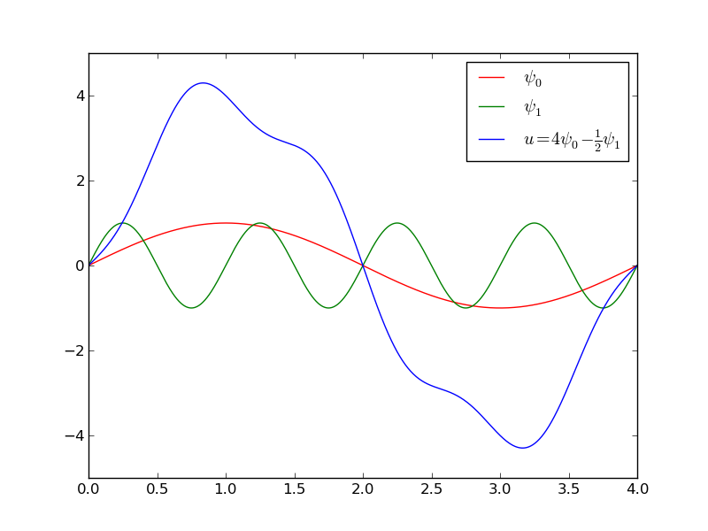
A function resulting from a weighted sum of two sine basis functions.
# #
#
#
#
#
#
#
#
#
#
#
#
#
#
#
#
#
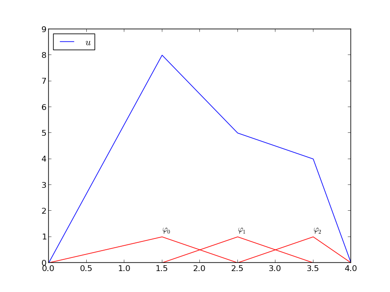
# A function resulting from a weighted sum of three local piecewise linear (hat) functions.
# #
#
#
#
# We first introduce the concepts of elements and nodes in a simplistic fashion.
# Later, we shall generalize the concept
# of an element, which is a necessary step before treating a wider class of
# approximations within the family of finite element methods.
# The generalization is also compatible with
# the concepts used in the [FEniCS](http://fenicsproject.org) finite
# element software.
#
# ## Elements and nodes
#
#
# Let $u$ and $f$ be defined on an interval $\Omega$. We divide $\Omega$
# into $N_e$ non-overlapping subintervals $\Omega^{(e)}$,
# $e=0,\ldots,N_e-1$:
#
#
#
# $$
# \begin{equation}
# \Omega = \Omega^{(0)}\cup \cdots \cup \Omega^{(N_e)}{\thinspace .} \label{_auto32} \tag{68}
# \end{equation}
# $$
# We shall for now refer to $\Omega^{(e)}$ as an *element*, identified
# by the unique number $e$. On each element we introduce a set of
# points called *nodes*. For now we assume that the nodes are uniformly
# spaced throughout the element and that the boundary points of the
# elements are also nodes. The nodes are given numbers both within an
# element and in the global domain. These are referred to as *local* and
# *global* node numbers, respectively. Local nodes are numbered with an
# index $r=0,\ldots,d$, while the $N_n$ global nodes are numbered as
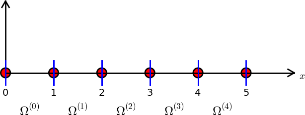
# $i=0,\ldots,N_n-1$. [Figure](#fem:approx:fe:def:elements:nodes:fig:P1) shows nodes as small
# circular disks and element boundaries as small vertical lines. Global
# node numbers appear under the nodes, but local node numbers are not
# shown. Since there are two nodes in each element, the local nodes are
# numbered 0 (left) and 1 (right) in each element.
#
#
#
#
#
#
#
#
#
#
# We first introduce the concepts of elements and nodes in a simplistic fashion.
# Later, we shall generalize the concept
# of an element, which is a necessary step before treating a wider class of
# approximations within the family of finite element methods.
# The generalization is also compatible with
# the concepts used in the [FEniCS](http://fenicsproject.org) finite
# element software.
#
# ## Elements and nodes
#
#
# Let $u$ and $f$ be defined on an interval $\Omega$. We divide $\Omega$
# into $N_e$ non-overlapping subintervals $\Omega^{(e)}$,
# $e=0,\ldots,N_e-1$:
#
#
#
# $$
# \begin{equation}
# \Omega = \Omega^{(0)}\cup \cdots \cup \Omega^{(N_e)}{\thinspace .} \label{_auto32} \tag{68}
# \end{equation}
# $$
# We shall for now refer to $\Omega^{(e)}$ as an *element*, identified
# by the unique number $e$. On each element we introduce a set of
# points called *nodes*. For now we assume that the nodes are uniformly
# spaced throughout the element and that the boundary points of the
# elements are also nodes. The nodes are given numbers both within an
# element and in the global domain. These are referred to as *local* and
# *global* node numbers, respectively. Local nodes are numbered with an
# index $r=0,\ldots,d$, while the $N_n$ global nodes are numbered as
# $i=0,\ldots,N_n-1$. [Figure](#fem:approx:fe:def:elements:nodes:fig:P1) shows nodes as small
# circular disks and element boundaries as small vertical lines. Global
# node numbers appear under the nodes, but local node numbers are not
# shown. Since there are two nodes in each element, the local nodes are
# numbered 0 (left) and 1 (right) in each element.
#
#
#
#
#
# Finite element mesh with 5 elements and 6 nodes.
# #
#
#
#
#
# Nodes and elements uniquely define a *finite element mesh*, which is
# our discrete representation of the domain in the computations. A
# common special case is that of a *uniformly partitioned mesh* where
# each element has the same length and the distance between nodes is
# constant. [Figure](#fem:approx:fe:def:elements:nodes:fig:P1) shows
# an example on a uniformly partitioned mesh. The strength of the finite
# element method (in contrast to the finite difference method) is that
# it is just as easy to work with a non-uniformly partitioned mesh in 3D as a
# uniformly partitioned mesh in 1D.
#
# ### Example
#
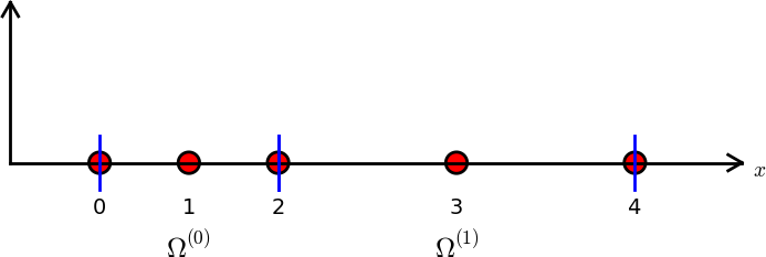
# On $\Omega =[0,1]$ we may introduce two elements,
# $\Omega^{(0)}=[0,0.4]$ and $\Omega^{(1)}=[0.4,1]$. Furthermore, let us
# introduce three nodes per element, equally spaced within each element.
# [Figure](#fem:approx:fe:def:elements:nodes:fig:P2) shows the mesh
# with $N_e=2$ elements and $N_n=2N_e+1=5$ nodes. A node's coordinate
# is denoted by $x_i$, where $i$ is either a global node number or a
# local one. In the latter case we also need to know the element number
# to uniquely define the node.
#
# The three nodes in element number 0 are $x_0=0$, $x_1=0.2$, and
# $x_2=0.4$. The local and global node numbers are here equal. In
# element number 1, we have the local nodes $x_0=0.4$, $x_1=0.7$, and
# $x_2=1$ and the corresponding global nodes $x_2=0.4$, $x_3=0.7$, and
# $x_4=1$. Note that the global node $x_2=0.4$ is shared by the two
# elements.
#
#
#
#
#
#
#
#
#
#
#
# Nodes and elements uniquely define a *finite element mesh*, which is
# our discrete representation of the domain in the computations. A
# common special case is that of a *uniformly partitioned mesh* where
# each element has the same length and the distance between nodes is
# constant. [Figure](#fem:approx:fe:def:elements:nodes:fig:P1) shows
# an example on a uniformly partitioned mesh. The strength of the finite
# element method (in contrast to the finite difference method) is that
# it is just as easy to work with a non-uniformly partitioned mesh in 3D as a
# uniformly partitioned mesh in 1D.
#
# ### Example
#
# On $\Omega =[0,1]$ we may introduce two elements,
# $\Omega^{(0)}=[0,0.4]$ and $\Omega^{(1)}=[0.4,1]$. Furthermore, let us
# introduce three nodes per element, equally spaced within each element.
# [Figure](#fem:approx:fe:def:elements:nodes:fig:P2) shows the mesh
# with $N_e=2$ elements and $N_n=2N_e+1=5$ nodes. A node's coordinate
# is denoted by $x_i$, where $i$ is either a global node number or a
# local one. In the latter case we also need to know the element number
# to uniquely define the node.
#
# The three nodes in element number 0 are $x_0=0$, $x_1=0.2$, and
# $x_2=0.4$. The local and global node numbers are here equal. In
# element number 1, we have the local nodes $x_0=0.4$, $x_1=0.7$, and
# $x_2=1$ and the corresponding global nodes $x_2=0.4$, $x_3=0.7$, and
# $x_4=1$. Note that the global node $x_2=0.4$ is shared by the two
# elements.
#
#
#
#
#
# Finite element mesh with 2 elements and 5 nodes.
# #
#
#
#
# For the purpose of implementation, we introduce two lists or arrays:
# `nodes` for storing the coordinates of the nodes, with the global node
# numbers as indices, and `elements` for holding the global node numbers
# in each element. By defining `elements` as a list of lists, where each
# sublist contains the global node numbers of one particular element,
# the indices of each sublist will correspond to local node numbers for
# that element. The `nodes` and `elements` lists for the sample mesh
# above take the form
# In[1]:
nodes = [0, 0.2, 0.4, 0.7, 1]
elements = [[0, 1, 2], [2, 3, 4]]
# Looking up the coordinate of, e.g., local node number 2 in element 1,
# is done by `nodes[elements[1][2]]` (recall that nodes and
# elements start their numbering at 0). The corresponding global node number
# is 4, so we could alternatively look up the coordinate as `nodes[4]`.
#
# The numbering of elements and nodes does not need to be regular.
# [Figure](#fem:approx:fe:def:elements:nodes:fig:P1:irregular) shows
# an example corresponding to
# In[2]:
nodes = [1.5, 5.5, 4.2, 0.3, 2.2, 3.1]
elements = [[2, 1], [4, 5], [0, 4], [3, 0], [5, 2]]
#
#
#
#
#
#
#
#
#
# For the purpose of implementation, we introduce two lists or arrays:
# `nodes` for storing the coordinates of the nodes, with the global node
# numbers as indices, and `elements` for holding the global node numbers
# in each element. By defining `elements` as a list of lists, where each
# sublist contains the global node numbers of one particular element,
# the indices of each sublist will correspond to local node numbers for
# that element. The `nodes` and `elements` lists for the sample mesh
# above take the form
# In[1]:
nodes = [0, 0.2, 0.4, 0.7, 1]
elements = [[0, 1, 2], [2, 3, 4]]
# Looking up the coordinate of, e.g., local node number 2 in element 1,
# is done by `nodes[elements[1][2]]` (recall that nodes and
# elements start their numbering at 0). The corresponding global node number
# is 4, so we could alternatively look up the coordinate as `nodes[4]`.
#
# The numbering of elements and nodes does not need to be regular.
# [Figure](#fem:approx:fe:def:elements:nodes:fig:P1:irregular) shows
# an example corresponding to
# In[2]:
nodes = [1.5, 5.5, 4.2, 0.3, 2.2, 3.1]
elements = [[2, 1], [4, 5], [0, 4], [3, 0], [5, 2]]
#
#
#
#
# Example on irregular numbering of elements and nodes.
# #
#
#
#
# ## The basis functions
#
# ### Construction principles
#
# Finite element basis functions are in this text recognized by
# the notation ${\varphi}_i(x)$, where the index (now in the beginning)
# corresponds to
# a global node number. Since ${\psi}_i$ is the symbol for basis
# functions in general in this text, the particular choice of
# finite element basis functions means that we take
# ${\psi}_i = {\varphi}_i$.
#
#
#
# Let $i$ be the global node number corresponding to local node $r$ in
# element number $e$ with $d+1$ local nodes. We distinguish between
# *internal* nodes in an element and *shared* nodes. The latter are
# nodes that are shared with the neighboring elements.
# The finite element basis functions ${\varphi}_i$
# are now defined as follows.
#
# * For an internal node, with global number $i$ and local number $r$,
# take ${\varphi}_i(x)$ to be the Lagrange
# polynomial that is 1 at the local node $r$ and zero
# at all other nodes in the element.
# The degree of the polynomial is $d$.
# On all other elements, ${\varphi}_i=0$.
#
# * For a shared node,
# let ${\varphi}_i$ be made up of the Lagrange polynomial on this element
# that is 1 at node $i$, combined with the Lagrange polynomial over
# the neighboring element that is also 1 at node $i$.
# On all other elements, ${\varphi}_i=0$.
#
# A visual impression of three such basis functions is given in
# [Figure](#fem:approx:fe:fig:P2). When solving differential equations,
# we need the derivatives of these basis functions as well, and the
# corresponding derivatives are shown in [Figure](#fem:approx:fe:fig:dP2).
# Note that the derivatives are highly discontinuous!
# In these figures,
# the domain $\Omega = [0,1]$ is divided into four equal-sized elements,
# each having three local nodes.
# The element boundaries are
# marked by vertical dashed lines and the nodes by small circles.
# The function ${\varphi}_2(x)$
# is composed of a quadratic Lagrange polynomial over element 0 and 1,
# ${\varphi}_3(x)$ corresponds to an internal node in element 1 and
# is therefore nonzero on this element only, while ${\varphi}_4(x)$
# is like ${\varphi}_2(x)$ composed to two Lagrange polynomials over two
# elements. Also observe that the basis function ${\varphi}_i$ is zero at
# all nodes, except at global node number $i$.
# We also remark that
# the shape of a basis function over an element is completely determined
# by the coordinates of the local nodes in the element.
#
#
#
#
#
#
#
#
#
#
#
#
#
#
#
# ## The basis functions
#
# ### Construction principles
#
# Finite element basis functions are in this text recognized by
# the notation ${\varphi}_i(x)$, where the index (now in the beginning)
# corresponds to
# a global node number. Since ${\psi}_i$ is the symbol for basis
# functions in general in this text, the particular choice of
# finite element basis functions means that we take
# ${\psi}_i = {\varphi}_i$.
#
#
#
# Let $i$ be the global node number corresponding to local node $r$ in
# element number $e$ with $d+1$ local nodes. We distinguish between
# *internal* nodes in an element and *shared* nodes. The latter are
# nodes that are shared with the neighboring elements.
# The finite element basis functions ${\varphi}_i$
# are now defined as follows.
#
# * For an internal node, with global number $i$ and local number $r$,
# take ${\varphi}_i(x)$ to be the Lagrange
# polynomial that is 1 at the local node $r$ and zero
# at all other nodes in the element.
# The degree of the polynomial is $d$.
# On all other elements, ${\varphi}_i=0$.
#
# * For a shared node,
# let ${\varphi}_i$ be made up of the Lagrange polynomial on this element
# that is 1 at node $i$, combined with the Lagrange polynomial over
# the neighboring element that is also 1 at node $i$.
# On all other elements, ${\varphi}_i=0$.
#
# A visual impression of three such basis functions is given in
# [Figure](#fem:approx:fe:fig:P2). When solving differential equations,
# we need the derivatives of these basis functions as well, and the
# corresponding derivatives are shown in [Figure](#fem:approx:fe:fig:dP2).
# Note that the derivatives are highly discontinuous!
# In these figures,
# the domain $\Omega = [0,1]$ is divided into four equal-sized elements,
# each having three local nodes.
# The element boundaries are
# marked by vertical dashed lines and the nodes by small circles.
# The function ${\varphi}_2(x)$
# is composed of a quadratic Lagrange polynomial over element 0 and 1,
# ${\varphi}_3(x)$ corresponds to an internal node in element 1 and
# is therefore nonzero on this element only, while ${\varphi}_4(x)$
# is like ${\varphi}_2(x)$ composed to two Lagrange polynomials over two
# elements. Also observe that the basis function ${\varphi}_i$ is zero at
# all nodes, except at global node number $i$.
# We also remark that
# the shape of a basis function over an element is completely determined
# by the coordinates of the local nodes in the element.
#
#
#
#
#
#
#
#
#
#
# Illustration of the piecewise quadratic basis functions associated with nodes in an element.
# #
#
#
#
#
#
#
#
#
#
#
#
#
#
#
#
#
# Illustration of the derivatives of the piecewise quadratic basis functions associated with nodes in an element.
# #
#
#
#
# ### Properties of ${\varphi}_i$
#
# The construction of basis functions according to the principles above
# lead to two important properties of ${\varphi}_i(x)$. First,
#
#
#
# $$
# \begin{equation}
# {\varphi}_i(x_{j}) =\delta_{ij},\quad \delta_{ij} =
# \left\lbrace\begin{array}{ll}
# 1, & i=j,\\
# 0, & i\neq j,
# \end{array}\right.
# \label{fem:approx:fe:phi:prop1} \tag{69}
# \end{equation}
# $$
# when $x_{j}$ is a node in the mesh with global node number $j$.
# The
# result ${\varphi}_i(x_{j}) =\delta_{ij}$ is obtained as
# the Lagrange polynomials are constructed to have
# exactly this property.
# The property also implies a convenient interpretation of $c_i$
# as the value of $u$ at node $i$. To show this, we expand $u$
# in the usual way as $\sum_jc_j{\psi}_j$ and choose ${\psi}_i = {\varphi}_i$:
# $$
# u(x_{i}) = \sum_{j\in{\mathcal{I}_s}} c_j {\psi}_j (x_{i}) =
# \sum_{j\in{\mathcal{I}_s}} c_j {\varphi}_j (x_{i}) = c_i {\varphi}_i (x_{i}) = c_i
# {\thinspace .}
# $$
# Because of this interpretation,
# the coefficient $c_i$ is by many named $u_i$ or $U_i$.
#
#
#
# Second,
# ${\varphi}_i(x)$ is mostly zero throughout the domain:
#
# * ${\varphi}_i(x) \neq 0$ only on those elements that contain global node $i$,
#
# * ${\varphi}_i(x){\varphi}_j(x) \neq 0$ if and only if $i$ and $j$ are global node
# numbers in the same element.
#
# Since $A_{i,j}$ is the integral of
# ${\varphi}_i{\varphi}_j$ it means that
# *most of the elements in the coefficient matrix will be zero*.
# We will come back to these properties and use
# them actively in computations to save memory and CPU time.
#
# In our example so far, each element has $d+1$ nodes, resulting in
# local Lagrange polynomials of degree $d$, but it is not a requirement to have
# the same $d$ value in each element.
#
# ## Example on quadratic finite element functions
#
# Let us set up the `nodes` and `elements` lists corresponding to the
# mesh implied by [Figure](#fem:approx:fe:fig:P2).
# [Figure](#fem:approx:fe:fig:P2:mesh) sketches the mesh and the
# numbering. We have
# In[3]:
nodes = [0, 0.125, 0.25, 0.375, 0.5, 0.625, 0.75, 0.875, 1.0]
elements = [[0, 1, 2], [2, 3, 4], [4, 5, 6], [6, 7, 8]]
#
#
#
#
#
#
#
#
#
# ### Properties of ${\varphi}_i$
#
# The construction of basis functions according to the principles above
# lead to two important properties of ${\varphi}_i(x)$. First,
#
#
#
# $$
# \begin{equation}
# {\varphi}_i(x_{j}) =\delta_{ij},\quad \delta_{ij} =
# \left\lbrace\begin{array}{ll}
# 1, & i=j,\\
# 0, & i\neq j,
# \end{array}\right.
# \label{fem:approx:fe:phi:prop1} \tag{69}
# \end{equation}
# $$
# when $x_{j}$ is a node in the mesh with global node number $j$.
# The
# result ${\varphi}_i(x_{j}) =\delta_{ij}$ is obtained as
# the Lagrange polynomials are constructed to have
# exactly this property.
# The property also implies a convenient interpretation of $c_i$
# as the value of $u$ at node $i$. To show this, we expand $u$
# in the usual way as $\sum_jc_j{\psi}_j$ and choose ${\psi}_i = {\varphi}_i$:
# $$
# u(x_{i}) = \sum_{j\in{\mathcal{I}_s}} c_j {\psi}_j (x_{i}) =
# \sum_{j\in{\mathcal{I}_s}} c_j {\varphi}_j (x_{i}) = c_i {\varphi}_i (x_{i}) = c_i
# {\thinspace .}
# $$
# Because of this interpretation,
# the coefficient $c_i$ is by many named $u_i$ or $U_i$.
#
#
#
# Second,
# ${\varphi}_i(x)$ is mostly zero throughout the domain:
#
# * ${\varphi}_i(x) \neq 0$ only on those elements that contain global node $i$,
#
# * ${\varphi}_i(x){\varphi}_j(x) \neq 0$ if and only if $i$ and $j$ are global node
# numbers in the same element.
#
# Since $A_{i,j}$ is the integral of
# ${\varphi}_i{\varphi}_j$ it means that
# *most of the elements in the coefficient matrix will be zero*.
# We will come back to these properties and use
# them actively in computations to save memory and CPU time.
#
# In our example so far, each element has $d+1$ nodes, resulting in
# local Lagrange polynomials of degree $d$, but it is not a requirement to have
# the same $d$ value in each element.
#
# ## Example on quadratic finite element functions
#
# Let us set up the `nodes` and `elements` lists corresponding to the
# mesh implied by [Figure](#fem:approx:fe:fig:P2).
# [Figure](#fem:approx:fe:fig:P2:mesh) sketches the mesh and the
# numbering. We have
# In[3]:
nodes = [0, 0.125, 0.25, 0.375, 0.5, 0.625, 0.75, 0.875, 1.0]
elements = [[0, 1, 2], [2, 3, 4], [4, 5, 6], [6, 7, 8]]
#
#
#
#
# Sketch of mesh with 4 elements and 3 nodes per element.
# #
#
#
#
#
# Let us explain mathematically how the basis functions are constructed
# according to the principles.
# Consider element number 1 in [Figure](#fem:approx:fe:fig:P2:mesh),
# $\Omega^{(1)}=[0.25, 0.5]$, with local nodes
# 0, 1, and 2 corresponding to global nodes 2, 3, and 4.
# The coordinates of these nodes are
# $0.25$, $0.375$, and $0.5$, respectively.
# We define three Lagrange
# polynomials on this element:
#
# 1. The polynomial that is 1 at local node 1
# (global node 3) makes up the basis function
# ${\varphi}_3(x)$ over this element,
# with ${\varphi}_3(x)=0$ outside the element.
#
# 2. The polynomial that is 1 at local node 0 (global node 2) is the "right
# part" of the global basis function
# ${\varphi}_2(x)$. The "left part" of ${\varphi}_2(x)$ consists of
# a Lagrange polynomial associated with local node 2 in
# the neighboring element $\Omega^{(0)}=[0, 0.25]$.
#
# 3. Finally, the polynomial that is 1 at local node 2 (global node 4)
# is the "left part" of the global basis function ${\varphi}_4(x)$.
# The "right part" comes from the Lagrange polynomial that is 1 at
# local node 0 in the neighboring element $\Omega^{(2)}=[0.5, 0.75]$.
#
# The specific mathematical form of the polynomials *over element* 1 is
# given by the formula ([56](#fem:approx:global:Lagrange:poly)):
# $$
# \begin{align*}
# {\varphi}_3(x) &= \frac{(x-0.25)(x-0.5)}{(0.375-0.25)(0.375-0.5)},\quad x\in\Omega^{(1)}\\
# {\varphi}_2(x) &= \frac{(x-0.375)(x-0.5)}{(0.25-0.375)(0.25-0.5)},\quad x\in\Omega^{(1)}\\
# {\varphi}_4(x) &= \frac{(x-0.25)(x-0.375)}{(0.5-0.25)(0.5-0.25)},\quad x\in\Omega^{(1)} .
# \end{align*}
# $$
# As mentioned earlier, any global basis function ${\varphi}_i(x)$ is zero
# on elements that do not contain the node with global node number $i$.
# Clearly, the property ([69](#fem:approx:fe:phi:prop1)) is easily
# verified, see for instance that ${\varphi}_3(0.375) = 1$ while
# ${\varphi}_3(0.25) = 0$ and ${\varphi}_3(0.5) = 0$.
#
# The other global functions associated with internal nodes,
# ${\varphi}_1$, ${\varphi}_5$, and ${\varphi}_7$, are all of the same shape
# as the drawn ${\varphi}_3$ in [Figure](#fem:approx:fe:fig:P2), while
# the global basis functions associated with shared nodes have the same
# shape as shown ${\varphi}_2$ and ${\varphi}_4$. If the elements were of
# different length, the basis functions would be stretched according to
# the element size and hence be different.
#
#
#
#
#
#
#
#
#
#
#
#
#
# ## Example on linear finite element functions
#
#
# [Figure](#fem:approx:fe:fig:P1) shows
# piecewise linear basis functions ($d=1$) (with derivatives in
# [Figure](#fem:approx:fe:fig:dP1)). These are mathematically
# simpler than the quadratic functions in the previous section, and one would
# therefore think that it is easier to understand the linear functions
# first. However, linear basis functions do not involve internal nodes
# and are therefore a special case of the general situation. That is why
# we think it is better to understand the construction of quadratic functions
# first, which easily generalize to any $d > 2$, and then look at the
# special case $d=1$.
#
#
#
#
#
#
#
#
#
#
#
# Let us explain mathematically how the basis functions are constructed
# according to the principles.
# Consider element number 1 in [Figure](#fem:approx:fe:fig:P2:mesh),
# $\Omega^{(1)}=[0.25, 0.5]$, with local nodes
# 0, 1, and 2 corresponding to global nodes 2, 3, and 4.
# The coordinates of these nodes are
# $0.25$, $0.375$, and $0.5$, respectively.
# We define three Lagrange
# polynomials on this element:
#
# 1. The polynomial that is 1 at local node 1
# (global node 3) makes up the basis function
# ${\varphi}_3(x)$ over this element,
# with ${\varphi}_3(x)=0$ outside the element.
#
# 2. The polynomial that is 1 at local node 0 (global node 2) is the "right
# part" of the global basis function
# ${\varphi}_2(x)$. The "left part" of ${\varphi}_2(x)$ consists of
# a Lagrange polynomial associated with local node 2 in
# the neighboring element $\Omega^{(0)}=[0, 0.25]$.
#
# 3. Finally, the polynomial that is 1 at local node 2 (global node 4)
# is the "left part" of the global basis function ${\varphi}_4(x)$.
# The "right part" comes from the Lagrange polynomial that is 1 at
# local node 0 in the neighboring element $\Omega^{(2)}=[0.5, 0.75]$.
#
# The specific mathematical form of the polynomials *over element* 1 is
# given by the formula ([56](#fem:approx:global:Lagrange:poly)):
# $$
# \begin{align*}
# {\varphi}_3(x) &= \frac{(x-0.25)(x-0.5)}{(0.375-0.25)(0.375-0.5)},\quad x\in\Omega^{(1)}\\
# {\varphi}_2(x) &= \frac{(x-0.375)(x-0.5)}{(0.25-0.375)(0.25-0.5)},\quad x\in\Omega^{(1)}\\
# {\varphi}_4(x) &= \frac{(x-0.25)(x-0.375)}{(0.5-0.25)(0.5-0.25)},\quad x\in\Omega^{(1)} .
# \end{align*}
# $$
# As mentioned earlier, any global basis function ${\varphi}_i(x)$ is zero
# on elements that do not contain the node with global node number $i$.
# Clearly, the property ([69](#fem:approx:fe:phi:prop1)) is easily
# verified, see for instance that ${\varphi}_3(0.375) = 1$ while
# ${\varphi}_3(0.25) = 0$ and ${\varphi}_3(0.5) = 0$.
#
# The other global functions associated with internal nodes,
# ${\varphi}_1$, ${\varphi}_5$, and ${\varphi}_7$, are all of the same shape
# as the drawn ${\varphi}_3$ in [Figure](#fem:approx:fe:fig:P2), while
# the global basis functions associated with shared nodes have the same
# shape as shown ${\varphi}_2$ and ${\varphi}_4$. If the elements were of
# different length, the basis functions would be stretched according to
# the element size and hence be different.
#
#
#
#
#
#
#
#
#
#
#
#
#
# ## Example on linear finite element functions
#
#
# [Figure](#fem:approx:fe:fig:P1) shows
# piecewise linear basis functions ($d=1$) (with derivatives in
# [Figure](#fem:approx:fe:fig:dP1)). These are mathematically
# simpler than the quadratic functions in the previous section, and one would
# therefore think that it is easier to understand the linear functions
# first. However, linear basis functions do not involve internal nodes
# and are therefore a special case of the general situation. That is why
# we think it is better to understand the construction of quadratic functions
# first, which easily generalize to any $d > 2$, and then look at the
# special case $d=1$.
#
#
#
#
#
# Illustration of the piecewise linear basis functions associated with nodes in an element.
# #
#
#
#
#
#
#
#
#
#
#
#
#
#
#
#
#
# Illustration of the derivatives of piecewise linear basis functions associated with nodes in an element.
# #
#
#
#
#
# We have the same four elements on $\Omega = [0,1]$. Now there are no
# internal nodes in the elements so that all basis functions are
# associated with shared nodes and hence made up of two Lagrange
# polynomials, one from each of the two neighboring elements. For
# example, ${\varphi}_1(x)$ results from the Lagrange polynomial in
# element 0 that is 1 at local node 1 and 0 at local node 0, combined
# with the Lagrange polynomial in element 1 that is 1 at local node 0
# and 0 at local node 1. The other basis functions are constructed
# similarly.
#
# Explicit mathematical formulas are needed for ${\varphi}_i(x)$ in
# computations. In the piecewise linear case, the formula
# ([56](#fem:approx:global:Lagrange:poly)) leads to
#
#
#
# $$
# \begin{equation}
# {\varphi}_i(x) = \left\lbrace\begin{array}{ll}
# 0, & x < x_{i-1},\\
# (x - x_{i-1})/(x_{i} - x_{i-1}),
# & x_{i-1} \leq x < x_{i},\\
# 1 -
# (x - x_{i})/(x_{i+1} - x_{i}),
# & x_{i} \leq x < x_{i+1},\\
# 0, & x\geq x_{i+1}{\thinspace .} \end{array}
# \right.
# \label{fem:approx:fe:phi:1:formula1} \tag{70}
# \end{equation}
# $$
# Here, $x_{j}$, $j=i-1,i,i+1$, denotes the coordinate of node $j$.
# For elements of equal length $h$ the formulas can be simplified to
#
#
#
# $$
# \begin{equation}
# {\varphi}_i(x) = \left\lbrace\begin{array}{ll}
# 0, & x < x_{i-1},\\
# (x - x_{i-1})/h,
# & x_{i-1} \leq x < x_{i},\\
# 1 -
# (x - x_{i})/h,
# & x_{i} \leq x < x_{i+1},\\
# 0, & x\geq x_{i+1} .
# \end{array}
# \right.
# \label{fem:approx:fe:phi:1:formula2} \tag{71}
# \end{equation}
# $$
# ## Example on cubic finite element functions
#
# Piecewise cubic basis functions can be defined by introducing four
# nodes per element. [Figure](#fem:approx:fe:fig:P3) shows
# examples on ${\varphi}_i(x)$, $i=3,4,5,6$, associated with element number 1.
# Note that ${\varphi}_4$ and ${\varphi}_5$ are nonzero only on element number 1,
# while
# ${\varphi}_3$ and ${\varphi}_6$ are made up of Lagrange polynomials on two
# neighboring elements.
#
#
#
#
#
#
#
#
#
#
#
# We have the same four elements on $\Omega = [0,1]$. Now there are no
# internal nodes in the elements so that all basis functions are
# associated with shared nodes and hence made up of two Lagrange
# polynomials, one from each of the two neighboring elements. For
# example, ${\varphi}_1(x)$ results from the Lagrange polynomial in
# element 0 that is 1 at local node 1 and 0 at local node 0, combined
# with the Lagrange polynomial in element 1 that is 1 at local node 0
# and 0 at local node 1. The other basis functions are constructed
# similarly.
#
# Explicit mathematical formulas are needed for ${\varphi}_i(x)$ in
# computations. In the piecewise linear case, the formula
# ([56](#fem:approx:global:Lagrange:poly)) leads to
#
#
#
# $$
# \begin{equation}
# {\varphi}_i(x) = \left\lbrace\begin{array}{ll}
# 0, & x < x_{i-1},\\
# (x - x_{i-1})/(x_{i} - x_{i-1}),
# & x_{i-1} \leq x < x_{i},\\
# 1 -
# (x - x_{i})/(x_{i+1} - x_{i}),
# & x_{i} \leq x < x_{i+1},\\
# 0, & x\geq x_{i+1}{\thinspace .} \end{array}
# \right.
# \label{fem:approx:fe:phi:1:formula1} \tag{70}
# \end{equation}
# $$
# Here, $x_{j}$, $j=i-1,i,i+1$, denotes the coordinate of node $j$.
# For elements of equal length $h$ the formulas can be simplified to
#
#
#
# $$
# \begin{equation}
# {\varphi}_i(x) = \left\lbrace\begin{array}{ll}
# 0, & x < x_{i-1},\\
# (x - x_{i-1})/h,
# & x_{i-1} \leq x < x_{i},\\
# 1 -
# (x - x_{i})/h,
# & x_{i} \leq x < x_{i+1},\\
# 0, & x\geq x_{i+1} .
# \end{array}
# \right.
# \label{fem:approx:fe:phi:1:formula2} \tag{71}
# \end{equation}
# $$
# ## Example on cubic finite element functions
#
# Piecewise cubic basis functions can be defined by introducing four
# nodes per element. [Figure](#fem:approx:fe:fig:P3) shows
# examples on ${\varphi}_i(x)$, $i=3,4,5,6$, associated with element number 1.
# Note that ${\varphi}_4$ and ${\varphi}_5$ are nonzero only on element number 1,
# while
# ${\varphi}_3$ and ${\varphi}_6$ are made up of Lagrange polynomials on two
# neighboring elements.
#
#
#
#
#
# Illustration of the piecewise cubic basis functions associated with nodes in an element.
# #
#
#
#
#
# We see that all the piecewise linear basis functions have the same
# "hat" shape. They are naturally referred to as *hat functions*,
# also called *chapeau functions*.
# The piecewise quadratic functions in [Figure](#fem:approx:fe:fig:P2)
# are seen to be of two types. "Rounded hats" associated with internal
# nodes in the elements and some more "sombrero" shaped hats associated
# with element boundary nodes. Higher-order basis functions also have
# hat-like shapes, but the functions have pronounced oscillations in addition,
# as illustrated in [Figure](#fem:approx:fe:fig:P3).
#
#
# A common terminology is to speak about *linear elements* as
# elements with two local nodes associated with
# piecewise linear basis functions. Similarly, *quadratic elements* and
# *cubic elements* refer to piecewise quadratic or cubic functions
# over elements with three or four local nodes, respectively.
# Alternative names, frequently used in the following, are **P1** for linear
# elements, **P2** for quadratic elements, and so forth: P$d$ signifies
# degree $d$ of the polynomial basis functions.
#
#
# ## Calculating the linear system
#
#
# The elements in the coefficient matrix and right-hand side are given
# by the formulas ([28](#fem:approx:Aij)) and ([29](#fem:approx:bi)), but
# now the choice of ${\psi}_i$ is ${\varphi}_i$. Consider P1 elements
# where ${\varphi}_i(x)$ is piecewise linear. Nodes and elements numbered
# consecutively from left to right in a uniformly partitioned mesh imply
# the nodes
# $$
# x_i=i h,\quad i=0,\ldots,N_n-1,
# $$
# and the elements
#
#
#
# $$
# \begin{equation}
# \Omega^{(i)} = [x_{i},x_{i+1}] = [i h, (i+1)h],\quad
# i=0,\ldots,N_e-1
# {\thinspace .}
# \label{_auto33} \tag{72}
# \end{equation}
# $$
# We have in this case $N_e$ elements and $N_n=N_e+1$ nodes.
# The parameter $N$ denotes the number of unknowns in the expansion
# for $u$, and with the P1 elements, $N=N_n$.
# The domain is $\Omega=[x_{0},x_{N}]$.
# The formula for ${\varphi}_i(x)$ is given by
# ([71](#fem:approx:fe:phi:1:formula2)) and a graphical illustration is
# provided in Figures [fem:approx:fe:fig:P1](#fem:approx:fe:fig:P1) and
# [fem:approx:fe:fig:phi:i:im1](#fem:approx:fe:fig:phi:i:im1).
#
#
#
#
#
#
#
#
#
#
#
#
#
#
#
#
#
#
#
# We see that all the piecewise linear basis functions have the same
# "hat" shape. They are naturally referred to as *hat functions*,
# also called *chapeau functions*.
# The piecewise quadratic functions in [Figure](#fem:approx:fe:fig:P2)
# are seen to be of two types. "Rounded hats" associated with internal
# nodes in the elements and some more "sombrero" shaped hats associated
# with element boundary nodes. Higher-order basis functions also have
# hat-like shapes, but the functions have pronounced oscillations in addition,
# as illustrated in [Figure](#fem:approx:fe:fig:P3).
#
#
# A common terminology is to speak about *linear elements* as
# elements with two local nodes associated with
# piecewise linear basis functions. Similarly, *quadratic elements* and
# *cubic elements* refer to piecewise quadratic or cubic functions
# over elements with three or four local nodes, respectively.
# Alternative names, frequently used in the following, are **P1** for linear
# elements, **P2** for quadratic elements, and so forth: P$d$ signifies
# degree $d$ of the polynomial basis functions.
#
#
# ## Calculating the linear system
#
#
# The elements in the coefficient matrix and right-hand side are given
# by the formulas ([28](#fem:approx:Aij)) and ([29](#fem:approx:bi)), but
# now the choice of ${\psi}_i$ is ${\varphi}_i$. Consider P1 elements
# where ${\varphi}_i(x)$ is piecewise linear. Nodes and elements numbered
# consecutively from left to right in a uniformly partitioned mesh imply
# the nodes
# $$
# x_i=i h,\quad i=0,\ldots,N_n-1,
# $$
# and the elements
#
#
#
# $$
# \begin{equation}
# \Omega^{(i)} = [x_{i},x_{i+1}] = [i h, (i+1)h],\quad
# i=0,\ldots,N_e-1
# {\thinspace .}
# \label{_auto33} \tag{72}
# \end{equation}
# $$
# We have in this case $N_e$ elements and $N_n=N_e+1$ nodes.
# The parameter $N$ denotes the number of unknowns in the expansion
# for $u$, and with the P1 elements, $N=N_n$.
# The domain is $\Omega=[x_{0},x_{N}]$.
# The formula for ${\varphi}_i(x)$ is given by
# ([71](#fem:approx:fe:phi:1:formula2)) and a graphical illustration is
# provided in Figures [fem:approx:fe:fig:P1](#fem:approx:fe:fig:P1) and
# [fem:approx:fe:fig:phi:i:im1](#fem:approx:fe:fig:phi:i:im1).
#
#
#
#
#
#
#
#
#
#
#
#
#
# Illustration of the piecewise linear basis functions corresponding to global node 2 and 3.
# #
#
#
#
# ### Calculating specific matrix entries
#
# Let us calculate the specific matrix entry $A_{2,3} = \int_\Omega
# {\varphi}_2{\varphi}_3{\, \mathrm{d}x}$. [Figure](#fem:approx:fe:fig:phi:2:3)
# shows what ${\varphi}_2$ and ${\varphi}_3$ look like. We realize
# from this figure that the product ${\varphi}_2{\varphi}_3\neq 0$
# only over element 2, which contains node 2 and 3.
# The particular formulas for ${\varphi}_{2}(x)$ and ${\varphi}_3(x)$ on
# $[x_{2},x_{3}]$ are found from ([71](#fem:approx:fe:phi:1:formula2)).
# The function
# ${\varphi}_3$ has positive slope over $[x_{2},x_{3}]$ and corresponds
# to the interval $[x_{i-1},x_{i}]$ in
# ([71](#fem:approx:fe:phi:1:formula2)). With $i=3$ we get
# $$
# {\varphi}_3(x) = (x-x_2)/h,
# $$
# while ${\varphi}_2(x)$ has negative slope over $[x_{2},x_{3}]$
# and corresponds to setting $i=2$ in ([71](#fem:approx:fe:phi:1:formula2)),
# $$
# {\varphi}_2(x) = 1- (x-x_2)/h{\thinspace .}
# $$
# We can now easily integrate,
# $$
# A_{2,3} = \int_\Omega {\varphi}_2{\varphi}_{3}{\, \mathrm{d}x} =
# \int_{x_{2}}^{x_{3}}
# \left(1 - \frac{x - x_{2}}{h}\right) \frac{x - x_{2}}{h}
# {\, \mathrm{d}x} = \frac{h}{6}{\thinspace .}
# $$
# The diagonal entry in the coefficient matrix becomes
# $$
# A_{2,2} =
# \int_{x_{1}}^{x_{2}}
# \left(\frac{x - x_{1}}{h}\right)^2{\, \mathrm{d}x} +
# \int_{x_{2}}^{x_{3}}
# \left(1 - \frac{x - x_{2}}{h}\right)^2{\, \mathrm{d}x}
# = \frac{2h}{3}{\thinspace .}
# $$
# The entry $A_{2,1}$ has an
# integral that is geometrically similar to the situation in
# [Figure](#fem:approx:fe:fig:phi:2:3), so we get
# $A_{2,1}=h/6$.
#
#
# ### Calculating a general row in the matrix
#
# We can now generalize the calculation of matrix entries to
# a general row number $i$. The entry
# $A_{i,i-1}=\int_\Omega{\varphi}_i{\varphi}_{i-1}{\, \mathrm{d}x}$ involves
# hat functions as depicted in
# [Figure](#fem:approx:fe:fig:phi:i:im1). Since the integral
# is geometrically identical to the situation with specific nodes
# 2 and 3, we realize that $A_{i,i-1}=A_{i,i+1}=h/6$ and
# $A_{i,i}=2h/3$. However, we can compute the integral directly
# too:
# $$
# \begin{align*}
# A_{i,i-1} &= \int_\Omega {\varphi}_i{\varphi}_{i-1}{\, \mathrm{d}x}\\
# &=
# \underbrace{\int_{x_{i-2}}^{x_{i-1}} {\varphi}_i{\varphi}_{i-1}{\, \mathrm{d}x}}_{{\varphi}_i=0} +
# \int_{x_{i-1}}^{x_{i}} {\varphi}_i{\varphi}_{i-1}{\, \mathrm{d}x} +
# \underbrace{\int_{x_{i}}^{x_{i+1}} {\varphi}_i{\varphi}_{i-1}{\, \mathrm{d}x}}_{{\varphi}_{i-1}=0}\\
# &= \int_{x_{i-1}}^{x_{i}}
# \underbrace{\left(\frac{x - x_{i}}{h}\right)}_{{\varphi}_i(x)}
# \underbrace{\left(1 - \frac{x - x_{i-1}}{h}\right)}_{{\varphi}_{i-1}(x)} {\, \mathrm{d}x} =
# \frac{h}{6}
# {\thinspace .}
# \end{align*}
# $$
# The particular formulas for ${\varphi}_{i-1}(x)$ and ${\varphi}_i(x)$ on
# $[x_{i-1},x_{i}]$ are found from ([71](#fem:approx:fe:phi:1:formula2)):
# ${\varphi}_i$ is the linear function with positive slope, corresponding
# to the interval $[x_{i-1},x_{i}]$ in
# ([71](#fem:approx:fe:phi:1:formula2)), while $\phi_{i-1}$ has a
# negative slope so the definition in interval
# $[x_{i},x_{i+1}]$ in ([71](#fem:approx:fe:phi:1:formula2)) must be
# used.
#
#
#
#
#
#
#
#
#
#
# ### Calculating specific matrix entries
#
# Let us calculate the specific matrix entry $A_{2,3} = \int_\Omega
# {\varphi}_2{\varphi}_3{\, \mathrm{d}x}$. [Figure](#fem:approx:fe:fig:phi:2:3)
# shows what ${\varphi}_2$ and ${\varphi}_3$ look like. We realize
# from this figure that the product ${\varphi}_2{\varphi}_3\neq 0$
# only over element 2, which contains node 2 and 3.
# The particular formulas for ${\varphi}_{2}(x)$ and ${\varphi}_3(x)$ on
# $[x_{2},x_{3}]$ are found from ([71](#fem:approx:fe:phi:1:formula2)).
# The function
# ${\varphi}_3$ has positive slope over $[x_{2},x_{3}]$ and corresponds
# to the interval $[x_{i-1},x_{i}]$ in
# ([71](#fem:approx:fe:phi:1:formula2)). With $i=3$ we get
# $$
# {\varphi}_3(x) = (x-x_2)/h,
# $$
# while ${\varphi}_2(x)$ has negative slope over $[x_{2},x_{3}]$
# and corresponds to setting $i=2$ in ([71](#fem:approx:fe:phi:1:formula2)),
# $$
# {\varphi}_2(x) = 1- (x-x_2)/h{\thinspace .}
# $$
# We can now easily integrate,
# $$
# A_{2,3} = \int_\Omega {\varphi}_2{\varphi}_{3}{\, \mathrm{d}x} =
# \int_{x_{2}}^{x_{3}}
# \left(1 - \frac{x - x_{2}}{h}\right) \frac{x - x_{2}}{h}
# {\, \mathrm{d}x} = \frac{h}{6}{\thinspace .}
# $$
# The diagonal entry in the coefficient matrix becomes
# $$
# A_{2,2} =
# \int_{x_{1}}^{x_{2}}
# \left(\frac{x - x_{1}}{h}\right)^2{\, \mathrm{d}x} +
# \int_{x_{2}}^{x_{3}}
# \left(1 - \frac{x - x_{2}}{h}\right)^2{\, \mathrm{d}x}
# = \frac{2h}{3}{\thinspace .}
# $$
# The entry $A_{2,1}$ has an
# integral that is geometrically similar to the situation in
# [Figure](#fem:approx:fe:fig:phi:2:3), so we get
# $A_{2,1}=h/6$.
#
#
# ### Calculating a general row in the matrix
#
# We can now generalize the calculation of matrix entries to
# a general row number $i$. The entry
# $A_{i,i-1}=\int_\Omega{\varphi}_i{\varphi}_{i-1}{\, \mathrm{d}x}$ involves
# hat functions as depicted in
# [Figure](#fem:approx:fe:fig:phi:i:im1). Since the integral
# is geometrically identical to the situation with specific nodes
# 2 and 3, we realize that $A_{i,i-1}=A_{i,i+1}=h/6$ and
# $A_{i,i}=2h/3$. However, we can compute the integral directly
# too:
# $$
# \begin{align*}
# A_{i,i-1} &= \int_\Omega {\varphi}_i{\varphi}_{i-1}{\, \mathrm{d}x}\\
# &=
# \underbrace{\int_{x_{i-2}}^{x_{i-1}} {\varphi}_i{\varphi}_{i-1}{\, \mathrm{d}x}}_{{\varphi}_i=0} +
# \int_{x_{i-1}}^{x_{i}} {\varphi}_i{\varphi}_{i-1}{\, \mathrm{d}x} +
# \underbrace{\int_{x_{i}}^{x_{i+1}} {\varphi}_i{\varphi}_{i-1}{\, \mathrm{d}x}}_{{\varphi}_{i-1}=0}\\
# &= \int_{x_{i-1}}^{x_{i}}
# \underbrace{\left(\frac{x - x_{i}}{h}\right)}_{{\varphi}_i(x)}
# \underbrace{\left(1 - \frac{x - x_{i-1}}{h}\right)}_{{\varphi}_{i-1}(x)} {\, \mathrm{d}x} =
# \frac{h}{6}
# {\thinspace .}
# \end{align*}
# $$
# The particular formulas for ${\varphi}_{i-1}(x)$ and ${\varphi}_i(x)$ on
# $[x_{i-1},x_{i}]$ are found from ([71](#fem:approx:fe:phi:1:formula2)):
# ${\varphi}_i$ is the linear function with positive slope, corresponding
# to the interval $[x_{i-1},x_{i}]$ in
# ([71](#fem:approx:fe:phi:1:formula2)), while $\phi_{i-1}$ has a
# negative slope so the definition in interval
# $[x_{i},x_{i+1}]$ in ([71](#fem:approx:fe:phi:1:formula2)) must be
# used.
#
#
#
#
#
# Illustration of two neighboring linear (hat) functions with general node numbers.
# #
#
#
#
#
# The first and last row of the coefficient matrix lead to slightly
# different integrals:
# $$
# A_{0,0} = \int_\Omega {\varphi}_0^2{\, \mathrm{d}x} = \int_{x_{0}}^{x_{1}}
# \left(1 - \frac{x-x_0}{h}\right)^2{\, \mathrm{d}x} = \frac{h}{3}{\thinspace .}
# $$
# Similarly, $A_{N,N}$ involves an integral over only one element
# and hence equals $h/3$.
#
#
#
#
#
#
#
#
#
#
#
# The first and last row of the coefficient matrix lead to slightly
# different integrals:
# $$
# A_{0,0} = \int_\Omega {\varphi}_0^2{\, \mathrm{d}x} = \int_{x_{0}}^{x_{1}}
# \left(1 - \frac{x-x_0}{h}\right)^2{\, \mathrm{d}x} = \frac{h}{3}{\thinspace .}
# $$
# Similarly, $A_{N,N}$ involves an integral over only one element
# and hence equals $h/3$.
#
#
#
#
#
# Right-hand side integral with the product of a basis function and the given function to approximate.
# #
#
#
#
#
# The general formula for $b_i$,
# see [Figure](#fem:approx:fe:fig:phi:i:f), is now easy to set up
#
#
#
# $$
# \begin{equation}
# b_i = \int_\Omega{\varphi}_i(x)f(x){\, \mathrm{d}x}
# = \int_{x_{i-1}}^{x_{i}} \frac{x - x_{i-1}}{h} f(x){\, \mathrm{d}x}
# + \int_{x_{i}}^{x_{i+1}} \left(1 - \frac{x - x_{i}}{h}\right) f(x)
# {\, \mathrm{d}x}{\thinspace .}
# \label{fem:approx:fe:bi:formula1} \tag{73}
# \end{equation}
# $$
# We remark that the above formula applies to internal nodes (living at the interface between two elements)
# and that for the nodes on the boundaries only one integral needs to be computed.
#
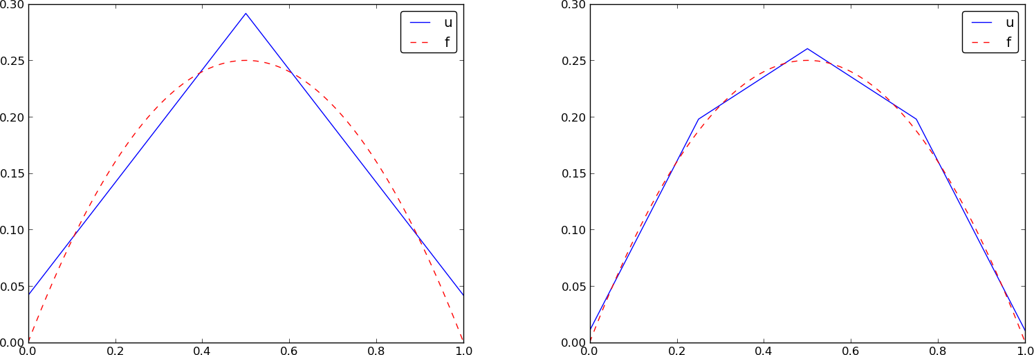
# We need a specific $f(x)$ function to compute these integrals.
# With $f(x)=x(1-x)$ and
# two equal-sized elements in $\Omega=[0,1]$, one gets
# $$
# A = \frac{h}{6}\left(\begin{array}{ccc}
# 2 & 1 & 0\\
# 1 & 4 & 1\\
# 0 & 1 & 2
# \end{array}\right),\quad
# b = \frac{h^2}{12}\left(\begin{array}{c}
# 2 - h\\
# 12 - 14h\\
# 10 -17h
# \end{array}\right){\thinspace .}
# $$
# The solution becomes
# $$
# c_0 = \frac{h^2}{6},\quad c_1 = h - \frac{5}{6}h^2,\quad
# c_2 = 2h - \frac{23}{6}h^2{\thinspace .}
# $$
# The resulting function
# $$
# u(x)=c_0{\varphi}_0(x) + c_1{\varphi}_1(x) + c_2{\varphi}_2(x)
# $$
# is displayed in [Figure](#fem:approx:fe:fig:ls:P1:2:4) (left).
# Doubling the number of elements to four leads to the improved
# approximation in the right part of [Figure](#fem:approx:fe:fig:ls:P1:2:4).
#
#
#
#
#
#
#
#
#
#
#
# The general formula for $b_i$,
# see [Figure](#fem:approx:fe:fig:phi:i:f), is now easy to set up
#
#
#
# $$
# \begin{equation}
# b_i = \int_\Omega{\varphi}_i(x)f(x){\, \mathrm{d}x}
# = \int_{x_{i-1}}^{x_{i}} \frac{x - x_{i-1}}{h} f(x){\, \mathrm{d}x}
# + \int_{x_{i}}^{x_{i+1}} \left(1 - \frac{x - x_{i}}{h}\right) f(x)
# {\, \mathrm{d}x}{\thinspace .}
# \label{fem:approx:fe:bi:formula1} \tag{73}
# \end{equation}
# $$
# We remark that the above formula applies to internal nodes (living at the interface between two elements)
# and that for the nodes on the boundaries only one integral needs to be computed.
#
# We need a specific $f(x)$ function to compute these integrals.
# With $f(x)=x(1-x)$ and
# two equal-sized elements in $\Omega=[0,1]$, one gets
# $$
# A = \frac{h}{6}\left(\begin{array}{ccc}
# 2 & 1 & 0\\
# 1 & 4 & 1\\
# 0 & 1 & 2
# \end{array}\right),\quad
# b = \frac{h^2}{12}\left(\begin{array}{c}
# 2 - h\\
# 12 - 14h\\
# 10 -17h
# \end{array}\right){\thinspace .}
# $$
# The solution becomes
# $$
# c_0 = \frac{h^2}{6},\quad c_1 = h - \frac{5}{6}h^2,\quad
# c_2 = 2h - \frac{23}{6}h^2{\thinspace .}
# $$
# The resulting function
# $$
# u(x)=c_0{\varphi}_0(x) + c_1{\varphi}_1(x) + c_2{\varphi}_2(x)
# $$
# is displayed in [Figure](#fem:approx:fe:fig:ls:P1:2:4) (left).
# Doubling the number of elements to four leads to the improved
# approximation in the right part of [Figure](#fem:approx:fe:fig:ls:P1:2:4).
#
#
#
#
#
# Least squares approximation of a parabola using 2 (left) and 4 (right) P1 elements.
# #
#
#
#
#
#
# ## Assembly of elementwise computations
#
#
# Our integral computations so far have been straightforward. However,
# with higher-degree polynomials and in higher dimensions (2D and 3D),
# integrating in the physical domain gets increasingly complicated. Instead,
# integrating over one element at a time, and transforming each element
# to a common standardized geometry in a new reference coordinate system,
# is technically easier. Almost all computer codes employ a finite element
# algorithm that calculates the linear system by integrating over one
# element at a time. We shall therefore explain this algorithm next.
# The amount of details might be overwhelming during a first reading, but
# once all those details are done right, one has a general
# finite element algorithm that can be applied to all sorts of elements,
# in any space dimension, no matter how geometrically complicated the domain
# is.
#
#
# ### The element matrix
#
# We start by splitting
# the integral over $\Omega$ into a sum of contributions from
# each element:
#
#
#
# $$
# \begin{equation}
# A_{i,j} = \int_\Omega{\varphi}_i{\varphi}_j {\, \mathrm{d}x} = \sum_{e} A^{(e)}_{i,j},\quad
# A^{(e)}_{i,j}=\int_{\Omega^{(e)}} {\varphi}_i{\varphi}_j {\, \mathrm{d}x}
# {\thinspace .}
# \label{fem:approx:fe:elementwise:Asplit} \tag{74}
# \end{equation}
# $$
# Now, $A^{(e)}_{i,j}\neq 0$, if and only if, $i$ and $j$ are nodes in element
# $e$ (look at [Figure](#fem:approx:fe:fig:phi:i:im1) to realize this
# property, but the result also holds for all types of elements).
# Introduce $i=q(e,r)$ as the mapping of local node number $r$ in element
# $e$ to the global node number $i$. This is just a short mathematical notation
# for the expression `i=elements[e][r]` in a program.
# Let $r$ and $s$ be the local node numbers corresponding to the global
# node numbers $i=q(e,r)$ and
# $j=q(e,s)$. With $d+1$ nodes per element, all the nonzero matrix entries
# in $A^{(e)}_{i,j}$ arise from the integrals involving basis functions with
# indices corresponding to the global node numbers in element number $e$:
# $$
# \int_{\Omega^{(e)}}{\varphi}_{q(e,r)}{\varphi}_{q(e,s)} {\, \mathrm{d}x},
# \quad r,s=0,\ldots, d{\thinspace .}
# $$
# These contributions can be collected in a $(d+1)\times (d+1)$ matrix known as
# the *element matrix*. Let ${I_d}=\{0,\ldots,d\}$ be the valid indices
# of $r$ and $s$.
# We introduce the notation
# $$
# \tilde A^{(e)} = \{ \tilde A^{(e)}_{r,s}\},\quad
# r,s\in{I_d},
# $$
# for the element matrix. For P1 elements ($d=2$) we have
# $$
# \tilde A^{(e)} = \left\lbrack\begin{array}{ll}
# \tilde A^{(e)}_{0,0} & \tilde A^{(e)}_{0,1}\\
# \tilde A^{(e)}_{1,0} & \tilde A^{(e)}_{1,1}
# \end{array}\right\rbrack
# {\thinspace .}
# $$
# while P2 elements have a $3\times 3$ element matrix:
# $$
# \tilde A^{(e)} = \left\lbrack\begin{array}{lll}
# \tilde A^{(e)}_{0,0} & \tilde A^{(e)}_{0,1} & \tilde A^{(e)}_{0,2}\\
# \tilde A^{(e)}_{1,0} & \tilde A^{(e)}_{1,1} & \tilde A^{(e)}_{1,2}\\
# \tilde A^{(e)}_{2,0} & \tilde A^{(e)}_{2,1} & \tilde A^{(e)}_{2,2}
# \end{array}\right\rbrack
# {\thinspace .}
# $$
# ### Assembly of element matrices
#
# Given the numbers $\tilde A^{(e)}_{r,s}$,
# we should, according to ([74](#fem:approx:fe:elementwise:Asplit)),
# add the contributions to the global coefficient matrix by
#
#
#
# $$
# \begin{equation}
# A_{q(e,r),q(e,s)} := A_{q(e,r),q(e,s)} + \tilde A^{(e)}_{r,s},\quad
# r,s\in{I_d}{\thinspace .}
# \label{_auto34} \tag{75}
# \end{equation}
# $$
# This process of adding in elementwise contributions to the global matrix
# is called *finite element assembly* or simply *assembly*.
#
# [Figure](#fem:approx:fe:fig:assembly:2x2) illustrates how element matrices
# for elements with two nodes are added into the global matrix.
# More specifically, the figure shows how the element matrix associated with
# elements 1 and 2 assembled, assuming that global nodes are numbered
# from left to right in the domain. With regularly numbered P3 elements, where
# the element matrices have size $4\times 4$, the assembly of elements 1 and 2
# are sketched in [Figure](#fem:approx:fe:fig:assembly:4x4).
#
#
#
#
#
#
#
#
#
#
#
#
# ## Assembly of elementwise computations
#
#
# Our integral computations so far have been straightforward. However,
# with higher-degree polynomials and in higher dimensions (2D and 3D),
# integrating in the physical domain gets increasingly complicated. Instead,
# integrating over one element at a time, and transforming each element
# to a common standardized geometry in a new reference coordinate system,
# is technically easier. Almost all computer codes employ a finite element
# algorithm that calculates the linear system by integrating over one
# element at a time. We shall therefore explain this algorithm next.
# The amount of details might be overwhelming during a first reading, but
# once all those details are done right, one has a general
# finite element algorithm that can be applied to all sorts of elements,
# in any space dimension, no matter how geometrically complicated the domain
# is.
#
#
# ### The element matrix
#
# We start by splitting
# the integral over $\Omega$ into a sum of contributions from
# each element:
#
#
#
# $$
# \begin{equation}
# A_{i,j} = \int_\Omega{\varphi}_i{\varphi}_j {\, \mathrm{d}x} = \sum_{e} A^{(e)}_{i,j},\quad
# A^{(e)}_{i,j}=\int_{\Omega^{(e)}} {\varphi}_i{\varphi}_j {\, \mathrm{d}x}
# {\thinspace .}
# \label{fem:approx:fe:elementwise:Asplit} \tag{74}
# \end{equation}
# $$
# Now, $A^{(e)}_{i,j}\neq 0$, if and only if, $i$ and $j$ are nodes in element
# $e$ (look at [Figure](#fem:approx:fe:fig:phi:i:im1) to realize this
# property, but the result also holds for all types of elements).
# Introduce $i=q(e,r)$ as the mapping of local node number $r$ in element
# $e$ to the global node number $i$. This is just a short mathematical notation
# for the expression `i=elements[e][r]` in a program.
# Let $r$ and $s$ be the local node numbers corresponding to the global
# node numbers $i=q(e,r)$ and
# $j=q(e,s)$. With $d+1$ nodes per element, all the nonzero matrix entries
# in $A^{(e)}_{i,j}$ arise from the integrals involving basis functions with
# indices corresponding to the global node numbers in element number $e$:
# $$
# \int_{\Omega^{(e)}}{\varphi}_{q(e,r)}{\varphi}_{q(e,s)} {\, \mathrm{d}x},
# \quad r,s=0,\ldots, d{\thinspace .}
# $$
# These contributions can be collected in a $(d+1)\times (d+1)$ matrix known as
# the *element matrix*. Let ${I_d}=\{0,\ldots,d\}$ be the valid indices
# of $r$ and $s$.
# We introduce the notation
# $$
# \tilde A^{(e)} = \{ \tilde A^{(e)}_{r,s}\},\quad
# r,s\in{I_d},
# $$
# for the element matrix. For P1 elements ($d=2$) we have
# $$
# \tilde A^{(e)} = \left\lbrack\begin{array}{ll}
# \tilde A^{(e)}_{0,0} & \tilde A^{(e)}_{0,1}\\
# \tilde A^{(e)}_{1,0} & \tilde A^{(e)}_{1,1}
# \end{array}\right\rbrack
# {\thinspace .}
# $$
# while P2 elements have a $3\times 3$ element matrix:
# $$
# \tilde A^{(e)} = \left\lbrack\begin{array}{lll}
# \tilde A^{(e)}_{0,0} & \tilde A^{(e)}_{0,1} & \tilde A^{(e)}_{0,2}\\
# \tilde A^{(e)}_{1,0} & \tilde A^{(e)}_{1,1} & \tilde A^{(e)}_{1,2}\\
# \tilde A^{(e)}_{2,0} & \tilde A^{(e)}_{2,1} & \tilde A^{(e)}_{2,2}
# \end{array}\right\rbrack
# {\thinspace .}
# $$
# ### Assembly of element matrices
#
# Given the numbers $\tilde A^{(e)}_{r,s}$,
# we should, according to ([74](#fem:approx:fe:elementwise:Asplit)),
# add the contributions to the global coefficient matrix by
#
#
#
# $$
# \begin{equation}
# A_{q(e,r),q(e,s)} := A_{q(e,r),q(e,s)} + \tilde A^{(e)}_{r,s},\quad
# r,s\in{I_d}{\thinspace .}
# \label{_auto34} \tag{75}
# \end{equation}
# $$
# This process of adding in elementwise contributions to the global matrix
# is called *finite element assembly* or simply *assembly*.
#
# [Figure](#fem:approx:fe:fig:assembly:2x2) illustrates how element matrices
# for elements with two nodes are added into the global matrix.
# More specifically, the figure shows how the element matrix associated with
# elements 1 and 2 assembled, assuming that global nodes are numbered
# from left to right in the domain. With regularly numbered P3 elements, where
# the element matrices have size $4\times 4$, the assembly of elements 1 and 2
# are sketched in [Figure](#fem:approx:fe:fig:assembly:4x4).
#
#
#
#
#
# Illustration of matrix assembly: regularly numbered P1 elements.
# #
#
#
#
#
#
#
#
#
#
#
#
#
#
#
#
#
# Illustration of matrix assembly: regularly numbered P3 elements.
# #
#
#
#
# ### Assembly of irregularly numbered elements and nodes
#
# After assembly of element matrices corresponding to regularly numbered elements
# and nodes are understood, it is wise to study the assembly process for
# irregularly numbered elements and nodes. [Figure](#fem:approx:fe:def:elements:nodes:fig:P1:irregular) shows a mesh where the `elements` array, or $q(e,r)$
# mapping in mathematical notation, is given as
# In[4]:
elements = [[2, 1], [4, 5], [0, 4], [3, 0], [5, 2]]
# The associated assembly of element matrices 1 and 2 is sketched in
# [Figure](#fem:approx:fe:fig:assembly:irr2x2).
#
# We have created [animations](${fem_doc}/mov/fe_assembly.html) to illustrate the assembly of
# P1 and P3 elements with regular numbering as well as P1 elements with
# irregular numbering. The reader is encouraged to develop a
# "geometric" understanding of how element matrix entries are added to
# the global matrix. This understanding is crucial for hand
# computations with the finite element method.
#
#
#
#
#
#
#
#
#
#
#
#
#
#
#
# ### Assembly of irregularly numbered elements and nodes
#
# After assembly of element matrices corresponding to regularly numbered elements
# and nodes are understood, it is wise to study the assembly process for
# irregularly numbered elements and nodes. [Figure](#fem:approx:fe:def:elements:nodes:fig:P1:irregular) shows a mesh where the `elements` array, or $q(e,r)$
# mapping in mathematical notation, is given as
# In[4]:
elements = [[2, 1], [4, 5], [0, 4], [3, 0], [5, 2]]
# The associated assembly of element matrices 1 and 2 is sketched in
# [Figure](#fem:approx:fe:fig:assembly:irr2x2).
#
# We have created [animations](${fem_doc}/mov/fe_assembly.html) to illustrate the assembly of
# P1 and P3 elements with regular numbering as well as P1 elements with
# irregular numbering. The reader is encouraged to develop a
# "geometric" understanding of how element matrix entries are added to
# the global matrix. This understanding is crucial for hand
# computations with the finite element method.
#
#
#
#
#
#
#
#
#
#
# Illustration of matrix assembly: irregularly numbered P1 elements.
# #
#
#
#
#
#
#
# ### The element vector
#
# The right-hand side of the linear system is also computed elementwise:
#
#
#
# $$
# \begin{equation}
# b_i = \int_\Omega f(x){\varphi}_i(x) {\, \mathrm{d}x} = \sum_{e} b^{(e)}_{i},\quad
# b^{(e)}_{i}=\int_{\Omega^{(e)}} f(x){\varphi}_i(x){\, \mathrm{d}x}
# {\thinspace .} \label{_auto35} \tag{76}
# \end{equation}
# $$
# We observe that
# $b_i^{(e)}\neq 0$ if and only if global node $i$ is a node in element $e$
# (look at [Figure](#fem:approx:fe:fig:phi:i:f) to realize this property).
# With $d$ nodes per element we can collect the $d+1$ nonzero contributions
# $b_i^{(e)}$, for $i=q(e,r)$, $r\in{I_d}$, in an *element vector*
# $$
# \tilde b_r^{(e)}=\{ \tilde b_r^{(e)}\},\quad r\in{I_d}{\thinspace .}
# $$
# These contributions are added to the
# global right-hand side by an assembly process similar to that for the
# element matrices:
#
#
#
# $$
# \begin{equation}
# b_{q(e,r)} := b_{q(e,r)} + \tilde b^{(e)}_{r},\quad
# r\in{I_d}{\thinspace .} \label{_auto36} \tag{77}
# \end{equation}
# $$
# ## Mapping to a reference element
#
#
#
# Instead of computing the integrals
# $$
# \tilde A^{(e)}_{r,s} = \int_{\Omega^{(e)}}{\varphi}_{q(e,r)}(x){\varphi}_{q(e,s)}(x){\, \mathrm{d}x}
# $$
# over some element
# $\Omega^{(e)} = [x_L, x_R]$ in the physical coordinate system,
# it turns out that it is considerably easier and more convenient
# to map the element domain $[x_L, x_R]$
# to a standardized reference element domain $[-1,1]$ and compute all
# integrals over the same domain $[-1,1]$.
# We have now introduced
# $x_L$ and $x_R$ as the left and right boundary points of an arbitrary element.
# With a natural, regular numbering of nodes and elements from left to right
# through the domain, we have $x_L=x_{e}$ and $x_R=x_{e+1}$ for P1 elements.
#
# ### The coordinate transformation
#
# Let $X\in [-1,1]$ be the coordinate
# in the reference element. A linear mapping, also known as an affine mapping,
# from $X$ to $x$ can be written
#
#
#
# $$
# \begin{equation}
# x = \frac{1}{2} (x_L + x_R) + \frac{1}{2} (x_R - x_L)X{\thinspace .}
# \label{fem:approx:fe:affine:mapping} \tag{78}
# \end{equation}
# $$
# This relation can alternatively be expressed as
#
#
#
# $$
# \begin{equation}
# x = x_m + {\frac{1}{2}}hX,
# \label{fem:approx:fe:affine:mapping2} \tag{79}
# \end{equation}
# $$
# where we have introduced the element midpoint $x_m=(x_L+x_R)/2$ and
# the element length $h=x_R-x_L$.
#
# ### Formulas for the element matrix and vector entries
#
# Integrating over the reference element is a matter of just changing the
# integration variable from $x$ to $X$. Let
#
#
#
# $$
# \begin{equation}
# {\tilde{\varphi}}_r(X) = {\varphi}_{q(e,r)}(x(X))
# \label{_auto37} \tag{80}
# \end{equation}
# $$
# be the basis function associated with local node number $r$ in the
# reference element. Switching from $x$ to $X$ as integration variable,
# using the rules from calculus, results in
#
#
#
# $$
# \begin{equation}
# \tilde A^{(e)}_{r,s} =
# \int_{\Omega^{(e)}}{\varphi}_{q(e,r)}(x){\varphi}_{q(e,s)}(x){\, \mathrm{d}x}
# = \int_{-1}^1 {\tilde{\varphi}}_r(X){\tilde{\varphi}}_s(X)\frac{{\, \mathrm{d}x}}{{\, \mathrm{d}X}}{\, \mathrm{d}X}
# {\thinspace .}
# \label{_auto38} \tag{81}
# \end{equation}
# $$
# In 2D and 3D, ${\, \mathrm{d}x}$ is transformed to $\hbox{det} J{\, \mathrm{d}X}$, where $J$ is
# the Jacobian of the mapping from $x$ to $X$. In 1D,
# $\hbox{det} J{\, \mathrm{d}X} = {\, \mathrm{d}x}/{\, \mathrm{d}X} = h/2$. To obtain a uniform
# notation for 1D, 2D, and 3D problems we therefore replace
# ${\, \mathrm{d}x}/{\, \mathrm{d}X}$ by $\det J$ now.
# The integration over the reference element is then written as
#
#
#
# $$
# \begin{equation}
# \tilde A^{(e)}_{r,s}
# = \int_{-1}^1 {\tilde{\varphi}}_r(X){\tilde{\varphi}}_s(X)\det J\,{\, \mathrm{d}X}
# \label{fem:approx:fe:mapping:Ae} \tag{82}
# {\thinspace .}
# \end{equation}
# $$
# The corresponding formula for the element vector entries becomes
#
#
#
# $$
# \begin{equation}
# \tilde b^{(e)}_{r} = \int_{\Omega^{(e)}}f(x){\varphi}_{q(e,r)}(x){\, \mathrm{d}x}
# = \int_{-1}^1 f(x(X)){\tilde{\varphi}}_r(X)\det J\,{\, \mathrm{d}X}
# \label{fem:approx:fe:mapping:be} \tag{83}
# {\thinspace .}
# \end{equation}
# $$
# **Why reference elements?**
#
# The great advantage of using reference elements is that
# the formulas for the basis functions, ${\tilde{\varphi}}_r(X)$, are the
# same for all elements and independent of the element geometry
# (length and location in the mesh). The geometric information
# is "factored out" in the simple mapping formula and the associated
# $\det J$ quantity. Also, the integration domain is the same for
# all elements. All these features contribute to simplify computer
# codes and make them more general.
#
#
#
#
#
#
#
#
#
#
#
#
#
#
# ### Formulas for local basis functions
#
# The ${\tilde{\varphi}}_r(x)$ functions are simply the Lagrange
# polynomials defined through the local nodes in the reference element.
# For $d=1$ and two nodes per element, we have the linear Lagrange
# polynomials
#
#
#
# $$
# \begin{equation}
# {\tilde{\varphi}}_0(X) = \frac{1}{2} (1 - X) ,
# \label{fem:approx:fe:mapping:P1:phi0} \tag{84}
# \end{equation}
# $$
#
#
#
# $$
# \begin{equation}
# {\tilde{\varphi}}_1(X) = \frac{1}{2} (1 + X) .
# \label{fem:approx:fe:mapping:P1:phi1} \tag{85}
# \end{equation}
# $$
# Quadratic polynomials, $d=2$, have the formulas
#
#
#
# $$
# \begin{equation}
# {\tilde{\varphi}}_0(X) = \frac{1}{2} (X-1)X,
# \label{fem:approx:fe:mapping:P2:phi0} \tag{86}
# \end{equation}
# $$
#
#
#
# $$
# \begin{equation}
# {\tilde{\varphi}}_1(X) = 1 - X^2,
# \label{fem:approx:fe:mapping:P2:phi1} \tag{87}
# \end{equation}
# $$
#
#
#
# $$
# \begin{equation}
# {\tilde{\varphi}}_2(X) = \frac{1}{2} (X+1)X .
# \label{fem:approx:fe:mapping:P2:phi2} \tag{88}
# \end{equation}
# $$
# In general,
#
#
#
# $$
# \begin{equation}
# {\tilde{\varphi}}_r(X) = \prod_{s=0,s\neq r}^d \frac{X-X_{(s)}}{X_{(r)}-X_{(s)}},
# \label{_auto39} \tag{89}
# \end{equation}
# $$
# where $X_{(0)},\ldots,X_{(d)}$ are the coordinates of the local nodes in
# the reference element.
# These are normally uniformly spaced: $X_{(r)} = -1 + 2r/d$,
# $r\in{I_d}$.
#
#
#
# ## Example on integration over a reference element
#
#
# To illustrate the concepts from the previous section in a specific
# example, we now
# consider calculation of the element matrix and vector for a specific choice of
# $d$ and $f(x)$. A simple choice is $d=1$ (P1 elements) and $f(x)=x(1-x)$
# on $\Omega =[0,1]$. We have the general expressions
# ([82](#fem:approx:fe:mapping:Ae)) and ([83](#fem:approx:fe:mapping:be))
# for $\tilde A^{(e)}_{r,s}$ and $\tilde b^{(e)}_{r}$.
# Writing these out for the choices ([84](#fem:approx:fe:mapping:P1:phi0))
# and ([85](#fem:approx:fe:mapping:P1:phi1)), and using that $\det J = h/2$,
# we can do the following calculations of the element matrix entries:
# $$
# \tilde A^{(e)}_{0,0}
# = \int_{-1}^1 {\tilde{\varphi}}_0(X){\tilde{\varphi}}_0(X)\frac{h}{2} {\, \mathrm{d}X}\nonumber
# $$
#
#
#
# $$
# \begin{equation}
# =\int_{-1}^1 \frac{1}{2}(1-X)\frac{1}{2}(1-X) \frac{h}{2} {\, \mathrm{d}X} =
# \frac{h}{8}\int_{-1}^1 (1-X)^2 {\, \mathrm{d}X} = \frac{h}{3},
# \label{fem:approx:fe:intg:ref:Ae00} \tag{90}
# \end{equation}
# $$
# $$
# \tilde A^{(e)}_{1,0}
# = \int_{-1}^1 {\tilde{\varphi}}_1(X){\tilde{\varphi}}_0(X)\frac{h}{2} {\, \mathrm{d}X}\nonumber
# $$
#
#
#
# $$
# \begin{equation}
# =\int_{-1}^1 \frac{1}{2}(1+X)\frac{1}{2}(1-X) \frac{h}{2} {\, \mathrm{d}X} =
# \frac{h}{8}\int_{-1}^1 (1-X^2) {\, \mathrm{d}X} = \frac{h}{6},
# \label{fem:approx:fe:intg:ref:Ae10} \tag{91}
# \end{equation}
# $$
#
#
#
# $$
# \begin{equation}
# \tilde A^{(e)}_{0,1} = \tilde A^{(e)}_{1,0},
# \label{_auto40} \tag{92}
# \end{equation}
# $$
# $$
# \tilde A^{(e)}_{1,1}
# = \int_{-1}^1 {\tilde{\varphi}}_1(X){\tilde{\varphi}}_1(X)\frac{h}{2} {\, \mathrm{d}X}\nonumber
# $$
#
#
#
# $$
# \begin{equation}
# =\int_{-1}^1 \frac{1}{2}(1+X)\frac{1}{2}(1+X) \frac{h}{2} {\, \mathrm{d}X} =
# \frac{h}{8}\int_{-1}^1 (1+X)^2 {\, \mathrm{d}X} = \frac{h}{3}
# \label{fem:approx:fe:intg:ref:Ae11} \tag{93}
# {\thinspace .}
# \end{equation}
# $$
# The corresponding entries in the element vector becomes
# using ([79](#fem:approx:fe:affine:mapping2)))
# $$
# \tilde b^{(e)}_{0}
# = \int_{-1}^1 f(x(X)){\tilde{\varphi}}_0(X)\frac{h}{2} {\, \mathrm{d}X}\nonumber
# $$
# $$
# = \int_{-1}^1 (x_m + \frac{1}{2} hX)(1-(x_m + \frac{1}{2} hX))
# \frac{1}{2}(1-X)\frac{h}{2} {\, \mathrm{d}X} \nonumber
# $$
#
#
#
# $$
# \begin{equation}
# = - \frac{1}{24} h^{3} + \frac{1}{6} h^{2} x_{m} - \frac{1}{12} h^{2} - \frac{1}{2} h x_{m}^{2} + \frac{1}{2} h x_{m},
# \label{fem:approx:fe:intg:ref:be0} \tag{94}
# \end{equation}
# $$
# $$
# \tilde b^{(e)}_{1}
# = \int_{-1}^1 f(x(X)){\tilde{\varphi}}_1(X)\frac{h}{2} {\, \mathrm{d}X}\nonumber
# $$
# $$
# = \int_{-1}^1 (x_m + \frac{1}{2} hX)(1-(x_m + \frac{1}{2} hX))
# \frac{1}{2}(1+X)\frac{h}{2} {\, \mathrm{d}X} \nonumber
# $$
#
#
#
# $$
# \begin{equation}
# = - \frac{1}{24} h^{3} - \frac{1}{6} h^{2} x_{m} + \frac{1}{12} h^{2} -
# \frac{1}{2} h x_{m}^{2} + \frac{1}{2} h x_{m}
# {\thinspace .}
# \label{_auto41} \tag{95}
# \end{equation}
# $$
# In the last two expressions we have used the element midpoint $x_m$.
#
# Integration of lower-degree polynomials above is tedious,
# and higher-degree polynomials involve much more algebra, but `sympy`
# may help. For example, we can easily calculate
# ([90](#fem:approx:fe:intg:ref:Ae00)),
# ([91](#fem:approx:fe:intg:ref:Ae10)),
# and ([94](#fem:approx:fe:intg:ref:be0)) by
# In[5]:
import sympy as sym
x, x_m, h, X = sym.symbols('x x_m h X')
sym.integrate(h/8*(1-X)**2, (X, -1, 1))
# In[6]:
sym.integrate(h/8*(1+X)*(1-X), (X, -1, 1))
# In[7]:
x = x_m + h/2*X
b_0 = sym.integrate(h/4*x*(1-x)*(1-X), (X, -1, 1))
print(b_0)
# # Implementation
#
#
# Based on the experience from the previous example, it makes sense to
# write some code to automate the analytical integration process for any
# choice of finite element basis functions. In addition, we can automate
# the assembly process and the solution of the linear system. Another
# advantage is that the code for these purposes document all details of
# all steps in the finite element computational machinery. The complete
# code can be found in the module file [`fe_approx1D.py`](src/fe_approx1D.py).
#
#
# ## Integration
#
#
# First we need a Python function for
# defining ${\tilde{\varphi}}_r(X)$ in terms of a Lagrange polynomial
# of degree `d`:
# In[8]:
import sympy as sym
import numpy as np
def basis(d, point_distribution='uniform', symbolic=False):
"""
Return all local basis function phi as functions of the
local point X in a 1D element with d+1 nodes.
If symbolic=True, return symbolic expressions, else
return Python functions of X.
point_distribution can be 'uniform' or 'Chebyshev'.
"""
X = sym.symbols('X')
if d == 0:
phi_sym = [1]
else:
if point_distribution == 'uniform':
if symbolic:
# Compute symbolic nodes
h = sym.Rational(1, d) # node spacing
nodes = [2*i*h - 1 for i in range(d+1)]
else:
nodes = np.linspace(-1, 1, d+1)
elif point_distribution == 'Chebyshev':
# Just numeric nodes
nodes = Chebyshev_nodes(-1, 1, d)
phi_sym = [Lagrange_polynomial(X, r, nodes)
for r in range(d+1)]
# Transform to Python functions
phi_num = [sym.lambdify([X], phi_sym[r], modules='numpy')
for r in range(d+1)]
return phi_sym if symbolic else phi_num
def Lagrange_polynomial(x, i, points):
p = 1
for k in range(len(points)):
if k != i:
p *= (x - points[k])/(points[i] - points[k])
return p
# Observe how we construct the `phi_sym` list to be
# symbolic expressions for ${\tilde{\varphi}}_r(X)$ with `X` as a
# `Symbol` object from `sympy`. Also note that the
# `Lagrange_polynomial` function works with both symbolic and numeric variables.
#
# Now we can write the function that computes the element matrix
# with a list of symbolic expressions for ${\varphi}_r$
# (`phi = basis(d, symbolic=True)`):
# In[9]:
def element_matrix(phi, Omega_e, symbolic=True):
n = len(phi)
A_e = sym.zeros(n, n)
X = sym.Symbol('X')
if symbolic:
h = sym.Symbol('h')
else:
h = Omega_e[1] - Omega_e[0]
detJ = h/2 # dx/dX
for r in range(n):
for s in range(r, n):
A_e[r,s] = sym.integrate(phi[r]*phi[s]*detJ, (X, -1, 1))
A_e[s,r] = A_e[r,s]
return A_e
# In the symbolic case (`symbolic` is `True`),
# we introduce the element length as a symbol
# `h` in the computations. Otherwise, the real numerical value
# of the element interval `Omega_e`
# is used and the final matrix elements are numbers,
# not symbols.
# This functionality can be demonstrated:
# In[11]:
from src.fe_approx1D import *
phi = basis(d=1, symbolic=True)
phi
# In[12]:
element_matrix(phi, Omega_e=[0.1, 0.2], symbolic=True)
# In[13]:
element_matrix(phi, Omega_e=[0.1, 0.2], symbolic=False)
# The computation of the element vector is done by a similar
# procedure:
# In[16]:
def element_vector(f, phi, Omega_e, symbolic=True):
n = len(phi)
b_e = sym.zeros(n, 1)
# Make f a function of X
X = sym.Symbol('X')
if symbolic:
h = sym.Symbol('h')
else:
h = Omega_e[1] - Omega_e[0]
x = (Omega_e[0] + Omega_e[1])/2 + h/2*X # mapping
f = f.subs('x', x) # substitute mapping formula for x
detJ = h/2 # dx/dX
for r in range(n):
b_e[r] = sym.integrate(f*phi[r]*detJ, (X, -1, 1))
return b_e
# Here we need to replace the symbol `x` in the expression for `f`
# by the mapping formula such that `f` can be integrated
# in terms of $X$, cf. the formula
# $\tilde b^{(e)}_{r} = \int_{-1}^1 f(x(X)){\tilde{\varphi}}_r(X)\frac{h}{2}{\, \mathrm{d}X}$.
#
# The integration in the element matrix function involves only products
# of polynomials, which `sympy` can easily deal with, but for the
# right-hand side `sympy` may face difficulties with certain types of
# expressions `f`. The result of the integral is then an `Integral`
# object and not a number or expression
# as when symbolic integration is successful.
# It may therefore be wise to introduce a fall back to the numerical
# integration. The symbolic integration can also spend considerable time
# before reaching an unsuccessful conclusion, so we may also introduce a parameter
# `symbolic` to turn symbolic integration on and off:
# In[15]:
#DO NOT RUN THIS CELL
def element_vector(f, phi, Omega_e, symbolic=True):
...
if symbolic:
I = sym.integrate(f*phi[r]*detJ, (X, -1, 1))
if not symbolic or isinstance(I, sym.Integral):
h = Omega_e[1] - Omega_e[0] # Ensure h is numerical
detJ = h/2
integrand = sym.lambdify([X], f*phi[r]*detJ, 'mpmath')
I = mpmath.quad(integrand, [-1, 1])
b_e[r] = I
...
# Numerical integration requires that the symbolic
# integrand is converted
# to a plain Python function (`integrand`) and that
# the element length `h` is a real number.
#
#
# ## Linear system assembly and solution
#
#
# The complete algorithm
# for computing and assembling the elementwise contributions
# takes the following form
# In[17]:
def assemble(nodes, elements, phi, f, symbolic=True):
N_n, N_e = len(nodes), len(elements)
if symbolic:
A = sym.zeros(N_n, N_n)
b = sym.zeros(N_n, 1) # note: (N_n, 1) matrix
else:
A = np.zeros((N_n, N_n))
b = np.zeros(N_n)
for e in range(N_e):
Omega_e = [nodes[elements[e][0]], nodes[elements[e][-1]]]
A_e = element_matrix(phi, Omega_e, symbolic)
b_e = element_vector(f, phi, Omega_e, symbolic)
for r in range(len(elements[e])):
for s in range(len(elements[e])):
A[elements[e][r],elements[e][s]] += A_e[r,s]
b[elements[e][r]] += b_e[r]
return A, b
# The `nodes` and `elements` variables represent the finite
# element mesh as explained earlier.
#
# Given the coefficient matrix `A` and the right-hand side `b`,
# we can compute the coefficients $\left\{ {c}_j \right\}_{j\in{\mathcal{I}_s}}$ in the expansion
# $u(x)=\sum_jc_j{\varphi}_j$ as the solution vector `c` of the linear
# system:
# In[ ]:
#DO NOT RUN THIS CELL
if symbolic:
c = A.LUsolve(b)
else:
c = np.linalg.solve(A, b)
# When `A` and `b` are `sympy` arrays,
# the solution procedure implied by `A.LUsolve` is symbolic.
# Otherwise, `A` and `b` are `numpy` arrays and a standard
# numerical solver is called.
# The symbolic version is suited for small problems only
# (small $N$ values) since the calculation time becomes prohibitively large
# otherwise. Normally, the symbolic *integration* will be more time
# consuming in small problems than the symbolic *solution* of the linear system.
#
# ## Example on computing symbolic approximations
#
#
# We can exemplify the use of `assemble` on the computational
# case from the section [Calculating the linear system](#fem:approx:global:linearsystem) with
# two P1 elements (linear basis functions) on the domain $\Omega=[0,1]$.
# Let us first work with a symbolic element length:
# In[19]:
h, x = sym.symbols('h x')
nodes = [0, h, 2*h]
elements = [[0, 1], [1, 2]]
phi = basis(d=1, symbolic=True)
f = x*(1-x)
A, b = assemble(nodes, elements, phi, f, symbolic=True)
A
# In[20]:
b
# In[21]:
c = A.LUsolve(b)
c
# ## Using interpolation instead of least squares
#
#
# As an alternative to the least squares formulation,
# we may compute the `c` vector based on
# the interpolation method from the section "The interpolation (or collocation) principle",
# using finite element basis functions.
# Choosing the nodes as interpolation points, the method can be written as
# $$
# u(x_{i}) = \sum_{j\in{\mathcal{I}_s}} c_j{\varphi}_j(x_{i}) = f(x_{i}),\quad
# i\in{\mathcal{I}_s}{\thinspace .}
# $$
# The coefficient matrix $A_{i,j}={\varphi}_j(x_{i})$ becomes
# the identity matrix because basis function number $j$ vanishes
# at all nodes, except node $i$: ${\varphi}_j(x_{i})=\delta_{ij}$.
# Therefore, $c_i = f(x_{i})$.
#
# The associated `sympy` calculations are
# In[22]:
fn = sym.lambdify([x], f)
c = [fn(xc) for xc in nodes]
c
# These expressions are much simpler than those based on least squares
# or projection in combination with finite element basis functions.
# However, which of the two methods that is most appropriate for a given
# task is problem-dependent, so we need both methods in our toolbox.
#
# ## Example on computing numerical approximations
#
#
# The numerical computations corresponding to the
# symbolic ones in the section [Example on computing symbolic approximations](#fem:approx:fe:impl:ex1:symbolic)
# (still done by `sympy` and the `assemble` function) go as follows:
# In[23]:
nodes = [0, 0.5, 1]
elements = [[0, 1], [1, 2]]
phi = basis(d=1, symbolic=True)
x = sym.Symbol('x')
f = x*(1-x)
A, b = assemble(nodes, elements, phi, f, symbolic=False)
A
# In[24]:
b
# In[28]:
c = np.linalg.solve(A, b)
c
# The [`fe_approx1D`](fe_approx1D.py) module contains functions for generating the
# `nodes` and `elements` lists for equal-sized elements with
# any number of nodes per element. The coordinates in `nodes`
# can be expressed either through the element length symbol `h`
# (`symbolic=True`) or by real numbers (`symbolic=False`):
# In[26]:
nodes, elements = mesh_uniform(N_e=10, d=3, Omega=[0,1],
symbolic=True)
# There is also a function
# In[ ]:
#DO NOT RUN THIS CELL
def approximate(f, symbolic=False, d=1, N_e=4, filename='tmp.pdf'):
# which computes a mesh with `N_e` elements, basis functions of
# degree `d`, and approximates a given symbolic expression
# `f` by a finite element expansion $u(x) = \sum_jc_j{\varphi}_j(x)$.
# When `symbolic` is `False`, $u(x) = \sum_jc_j{\varphi}_j(x)$
# can be computed at a (large)
# number of points and plotted together with $f(x)$. The construction
# of the pointwise function $u$ from the solution vector `c` is done
# elementwise by evaluating $\sum_rc_r{\tilde{\varphi}}_r(X)$ at a (large)
# number of points in each element in the local coordinate system,
# and the discrete $(x,u)$ values on
# each element are stored in separate arrays that are finally
# concatenated to form a global array for $x$ and for $u$.
# The details are found in the `u_glob` function in
# [`fe_approx1D.py`](fe_approx1D.py).
#
#
#
# ## The structure of the coefficient matrix
#
#
# Let us first see how the global matrix looks if we assemble
# symbolic element matrices, expressed in terms of `h`, from
# several elements:
# In[31]:
from src.fe_approx1D_v1 import mesh_symbolic
d=1; N_e=8; Omega=[0,1] # 8 linear elements on [0,1]
phi = basis(d)
f = x*(1-x)
nodes, elements = mesh_symbolic(N_e, d, Omega)
A, b = assemble(nodes, elements, phi, f, symbolic=True)
A
# The reader is encouraged to assemble the element matrices by hand and verify
# this result, as this exercise will give a hands-on understanding of
# what the assembly is about. In general we have a coefficient matrix that is
# tridiagonal:
#
#
#
# $$
# \begin{equation}
# A = \frac{h}{6}
# \left(
# \begin{array}{cccccccccc}
# 2 & 1 & 0
# &\cdots & \cdots & \cdots & \cdots & \cdots & 0 \\
# 1 & 4 & 1 & \ddots & & & & & \vdots \\
# 0 & 1 & 4 & 1 &
# \ddots & & & & \vdots \\
# \vdots & \ddots & & \ddots & \ddots & 0 & & & \vdots \\
# \vdots & & \ddots & \ddots & \ddots & \ddots & \ddots & & \vdots \\
# \vdots & & & 0 & 1 & 4 & 1 & \ddots & \vdots \\
# \vdots & & & & \ddots & \ddots & \ddots &\ddots & 0 \\
# \vdots & & & & &\ddots & 1 & 4 & 1 \\
# 0 &\cdots & \cdots &\cdots & \cdots & \cdots & 0 & 1 & 2
# \end{array}
# \right)
# \label{fem:approx:fe:A:fullmat} \tag{96}
# \end{equation}
# $$
# The structure of the right-hand side is more difficult to reveal since
# it involves an assembly of elementwise integrals of
# $f(x(X)){\tilde{\varphi}}_r(X)h/2$, which obviously depend on the
# particular choice of $f(x)$.
# Numerical integration can give some insight into the nature of
# the right-hand side. For this purpose it
# is easier to look at the integration in $x$ coordinates, which
# gives the general formula ([73](#fem:approx:fe:bi:formula1)).
# For equal-sized elements of length $h$, we can apply the
# Trapezoidal rule at the global node points to arrive at
# $$
# b_i = h\left( \frac{1}{2} {\varphi}_i(x_{0})f(x_{0}) +
# \frac{1}{2} {\varphi}_i(x_{N})f(x_{N}) + \sum_{j=1}^{N-1}
# {\varphi}_i(x_{j})f(x_{j})\right),
# $$
# which leads to
#
#
#
# $$
# \begin{equation}
# b_i =
# \left\lbrace\begin{array}{ll}
# \frac{1}{2} hf(x_i),& i=0\hbox{ or }i=N,\\
# h f(x_i), & 1 \leq i \leq N-1
# \end{array}\right.
# \label{_auto42} \tag{97}
# \end{equation}
# $$
# The reason for this simple formula is just that ${\varphi}_i$ is either
# 0 or 1 at the nodes and 0 at all but one of them.
#
# Going to P2 elements (`d=2`) leads
# to the element matrix
#
#
#
# $$
# \begin{equation}
# A^{(e)} = \frac{h}{30}
# \left(\begin{array}{ccc}
# 4 & 2 & -1\\
# 2 & 16 & 2\\
# -1 & 2 & 4
# \end{array}\right),
# \label{_auto43} \tag{98}
# \end{equation}
# $$
# and the following global matrix, assembled here from four elements:
#
#
#
# $$
# \begin{equation}
# A = \frac{h}{30}
# \left(
# \begin{array}{ccccccccc}
# 4 & 2 & - 1 & 0
# & 0 & 0 & 0 & 0 & 0\\
# 2 & 16 & 2
# & 0 & 0 & 0 & 0 & 0 & 0\\- 1 & 2 &
# 8 & 2 & - 1 & 0 & 0 & 0 &
# 0\\0 & 0 & 2 & 16 & 2 & 0 & 0
# & 0 & 0\\0 & 0 & - 1 & 2 & 8
# & 2 & - 1 & 0 & 0\\0 & 0 & 0 & 0 &
# 2 & 16 & 2 & 0 & 0\\0 & 0 & 0
# & 0 & - 1 & 2 & 8 &
# 2 & - 1\\0 & 0 & 0 & 0 & 0 & 0 &
# 2 & 16 & 2\\0 & 0 & 0 & 0 & 0
# & 0 & - 1 & 2 & 4
# \end{array}
# \right) .
# \label{_auto44} \tag{99}
# \end{equation}
# $$
# In general, for $i$ odd we have the nonzero elements
# $$
# A_{i,i-2} = -1,\quad A_{i-1,i}=2,\quad A_{i,i} = 8,\quad A_{i+1,i}=2,
# \quad A_{i+2,i}=-1,
# $$
# multiplied by $h/30$, and for $i$ even we have the nonzero elements
# $$
# A_{i-1,i}=2,\quad A_{i,i} = 16,\quad A_{i+1,i}=2,
# $$
# multiplied by $h/30$. The rows with odd numbers correspond to
# nodes at the element boundaries and get contributions from two
# neighboring elements in the assembly process,
# while the even numbered rows correspond to
# internal nodes in the elements where only one element contributes
# to the values in the global matrix.
#
# ## Applications
#
#
# With the aid of the `approximate` function in the `fe_approx1D`
# module we can easily investigate the quality of various finite element
# approximations to some given functions. [Figure](#fem:approx:fe:x9:sin)
# shows how linear and quadratic elements approximate the polynomial
# $f(x)=x(1-x)^8$ on $\Omega =[0,1]$, using equal-sized elements.
# The results arise from the program
# In[1]:
import sympy as sym
from src.fe_approx1D import approximate
x = sym.Symbol('x')
approximate(f=x*(1-x)**8, symbolic=False, d=1, N_e=4)
approximate(f=x*(1-x)**8, symbolic=False, d=2, N_e=2)
approximate(f=x*(1-x)**8, symbolic=False, d=1, N_e=8)
approximate(f=x*(1-x)**8, symbolic=False, d=2, N_e=4)
# The quadratic functions are seen to be better than the linear ones for the same
# value of $N$, as we increase $N$. This observation has some generality:
# higher degree is not necessarily better on a coarse mesh, but it is as
# we refine the mesh and the function becomes properly resolved.
#
#
#
#
#
#
#
#
#
#
#
#
#
#
# ### The element vector
#
# The right-hand side of the linear system is also computed elementwise:
#
#
#
# $$
# \begin{equation}
# b_i = \int_\Omega f(x){\varphi}_i(x) {\, \mathrm{d}x} = \sum_{e} b^{(e)}_{i},\quad
# b^{(e)}_{i}=\int_{\Omega^{(e)}} f(x){\varphi}_i(x){\, \mathrm{d}x}
# {\thinspace .} \label{_auto35} \tag{76}
# \end{equation}
# $$
# We observe that
# $b_i^{(e)}\neq 0$ if and only if global node $i$ is a node in element $e$
# (look at [Figure](#fem:approx:fe:fig:phi:i:f) to realize this property).
# With $d$ nodes per element we can collect the $d+1$ nonzero contributions
# $b_i^{(e)}$, for $i=q(e,r)$, $r\in{I_d}$, in an *element vector*
# $$
# \tilde b_r^{(e)}=\{ \tilde b_r^{(e)}\},\quad r\in{I_d}{\thinspace .}
# $$
# These contributions are added to the
# global right-hand side by an assembly process similar to that for the
# element matrices:
#
#
#
# $$
# \begin{equation}
# b_{q(e,r)} := b_{q(e,r)} + \tilde b^{(e)}_{r},\quad
# r\in{I_d}{\thinspace .} \label{_auto36} \tag{77}
# \end{equation}
# $$
# ## Mapping to a reference element
#
#
#
# Instead of computing the integrals
# $$
# \tilde A^{(e)}_{r,s} = \int_{\Omega^{(e)}}{\varphi}_{q(e,r)}(x){\varphi}_{q(e,s)}(x){\, \mathrm{d}x}
# $$
# over some element
# $\Omega^{(e)} = [x_L, x_R]$ in the physical coordinate system,
# it turns out that it is considerably easier and more convenient
# to map the element domain $[x_L, x_R]$
# to a standardized reference element domain $[-1,1]$ and compute all
# integrals over the same domain $[-1,1]$.
# We have now introduced
# $x_L$ and $x_R$ as the left and right boundary points of an arbitrary element.
# With a natural, regular numbering of nodes and elements from left to right
# through the domain, we have $x_L=x_{e}$ and $x_R=x_{e+1}$ for P1 elements.
#
# ### The coordinate transformation
#
# Let $X\in [-1,1]$ be the coordinate
# in the reference element. A linear mapping, also known as an affine mapping,
# from $X$ to $x$ can be written
#
#
#
# $$
# \begin{equation}
# x = \frac{1}{2} (x_L + x_R) + \frac{1}{2} (x_R - x_L)X{\thinspace .}
# \label{fem:approx:fe:affine:mapping} \tag{78}
# \end{equation}
# $$
# This relation can alternatively be expressed as
#
#
#
# $$
# \begin{equation}
# x = x_m + {\frac{1}{2}}hX,
# \label{fem:approx:fe:affine:mapping2} \tag{79}
# \end{equation}
# $$
# where we have introduced the element midpoint $x_m=(x_L+x_R)/2$ and
# the element length $h=x_R-x_L$.
#
# ### Formulas for the element matrix and vector entries
#
# Integrating over the reference element is a matter of just changing the
# integration variable from $x$ to $X$. Let
#
#
#
# $$
# \begin{equation}
# {\tilde{\varphi}}_r(X) = {\varphi}_{q(e,r)}(x(X))
# \label{_auto37} \tag{80}
# \end{equation}
# $$
# be the basis function associated with local node number $r$ in the
# reference element. Switching from $x$ to $X$ as integration variable,
# using the rules from calculus, results in
#
#
#
# $$
# \begin{equation}
# \tilde A^{(e)}_{r,s} =
# \int_{\Omega^{(e)}}{\varphi}_{q(e,r)}(x){\varphi}_{q(e,s)}(x){\, \mathrm{d}x}
# = \int_{-1}^1 {\tilde{\varphi}}_r(X){\tilde{\varphi}}_s(X)\frac{{\, \mathrm{d}x}}{{\, \mathrm{d}X}}{\, \mathrm{d}X}
# {\thinspace .}
# \label{_auto38} \tag{81}
# \end{equation}
# $$
# In 2D and 3D, ${\, \mathrm{d}x}$ is transformed to $\hbox{det} J{\, \mathrm{d}X}$, where $J$ is
# the Jacobian of the mapping from $x$ to $X$. In 1D,
# $\hbox{det} J{\, \mathrm{d}X} = {\, \mathrm{d}x}/{\, \mathrm{d}X} = h/2$. To obtain a uniform
# notation for 1D, 2D, and 3D problems we therefore replace
# ${\, \mathrm{d}x}/{\, \mathrm{d}X}$ by $\det J$ now.
# The integration over the reference element is then written as
#
#
#
# $$
# \begin{equation}
# \tilde A^{(e)}_{r,s}
# = \int_{-1}^1 {\tilde{\varphi}}_r(X){\tilde{\varphi}}_s(X)\det J\,{\, \mathrm{d}X}
# \label{fem:approx:fe:mapping:Ae} \tag{82}
# {\thinspace .}
# \end{equation}
# $$
# The corresponding formula for the element vector entries becomes
#
#
#
# $$
# \begin{equation}
# \tilde b^{(e)}_{r} = \int_{\Omega^{(e)}}f(x){\varphi}_{q(e,r)}(x){\, \mathrm{d}x}
# = \int_{-1}^1 f(x(X)){\tilde{\varphi}}_r(X)\det J\,{\, \mathrm{d}X}
# \label{fem:approx:fe:mapping:be} \tag{83}
# {\thinspace .}
# \end{equation}
# $$
# **Why reference elements?**
#
# The great advantage of using reference elements is that
# the formulas for the basis functions, ${\tilde{\varphi}}_r(X)$, are the
# same for all elements and independent of the element geometry
# (length and location in the mesh). The geometric information
# is "factored out" in the simple mapping formula and the associated
# $\det J$ quantity. Also, the integration domain is the same for
# all elements. All these features contribute to simplify computer
# codes and make them more general.
#
#
#
#
#
#
#
#
#
#
#
#
#
#
# ### Formulas for local basis functions
#
# The ${\tilde{\varphi}}_r(x)$ functions are simply the Lagrange
# polynomials defined through the local nodes in the reference element.
# For $d=1$ and two nodes per element, we have the linear Lagrange
# polynomials
#
#
#
# $$
# \begin{equation}
# {\tilde{\varphi}}_0(X) = \frac{1}{2} (1 - X) ,
# \label{fem:approx:fe:mapping:P1:phi0} \tag{84}
# \end{equation}
# $$
#
#
#
# $$
# \begin{equation}
# {\tilde{\varphi}}_1(X) = \frac{1}{2} (1 + X) .
# \label{fem:approx:fe:mapping:P1:phi1} \tag{85}
# \end{equation}
# $$
# Quadratic polynomials, $d=2$, have the formulas
#
#
#
# $$
# \begin{equation}
# {\tilde{\varphi}}_0(X) = \frac{1}{2} (X-1)X,
# \label{fem:approx:fe:mapping:P2:phi0} \tag{86}
# \end{equation}
# $$
#
#
#
# $$
# \begin{equation}
# {\tilde{\varphi}}_1(X) = 1 - X^2,
# \label{fem:approx:fe:mapping:P2:phi1} \tag{87}
# \end{equation}
# $$
#
#
#
# $$
# \begin{equation}
# {\tilde{\varphi}}_2(X) = \frac{1}{2} (X+1)X .
# \label{fem:approx:fe:mapping:P2:phi2} \tag{88}
# \end{equation}
# $$
# In general,
#
#
#
# $$
# \begin{equation}
# {\tilde{\varphi}}_r(X) = \prod_{s=0,s\neq r}^d \frac{X-X_{(s)}}{X_{(r)}-X_{(s)}},
# \label{_auto39} \tag{89}
# \end{equation}
# $$
# where $X_{(0)},\ldots,X_{(d)}$ are the coordinates of the local nodes in
# the reference element.
# These are normally uniformly spaced: $X_{(r)} = -1 + 2r/d$,
# $r\in{I_d}$.
#
#
#
# ## Example on integration over a reference element
#
#
# To illustrate the concepts from the previous section in a specific
# example, we now
# consider calculation of the element matrix and vector for a specific choice of
# $d$ and $f(x)$. A simple choice is $d=1$ (P1 elements) and $f(x)=x(1-x)$
# on $\Omega =[0,1]$. We have the general expressions
# ([82](#fem:approx:fe:mapping:Ae)) and ([83](#fem:approx:fe:mapping:be))
# for $\tilde A^{(e)}_{r,s}$ and $\tilde b^{(e)}_{r}$.
# Writing these out for the choices ([84](#fem:approx:fe:mapping:P1:phi0))
# and ([85](#fem:approx:fe:mapping:P1:phi1)), and using that $\det J = h/2$,
# we can do the following calculations of the element matrix entries:
# $$
# \tilde A^{(e)}_{0,0}
# = \int_{-1}^1 {\tilde{\varphi}}_0(X){\tilde{\varphi}}_0(X)\frac{h}{2} {\, \mathrm{d}X}\nonumber
# $$
#
#
#
# $$
# \begin{equation}
# =\int_{-1}^1 \frac{1}{2}(1-X)\frac{1}{2}(1-X) \frac{h}{2} {\, \mathrm{d}X} =
# \frac{h}{8}\int_{-1}^1 (1-X)^2 {\, \mathrm{d}X} = \frac{h}{3},
# \label{fem:approx:fe:intg:ref:Ae00} \tag{90}
# \end{equation}
# $$
# $$
# \tilde A^{(e)}_{1,0}
# = \int_{-1}^1 {\tilde{\varphi}}_1(X){\tilde{\varphi}}_0(X)\frac{h}{2} {\, \mathrm{d}X}\nonumber
# $$
#
#
#
# $$
# \begin{equation}
# =\int_{-1}^1 \frac{1}{2}(1+X)\frac{1}{2}(1-X) \frac{h}{2} {\, \mathrm{d}X} =
# \frac{h}{8}\int_{-1}^1 (1-X^2) {\, \mathrm{d}X} = \frac{h}{6},
# \label{fem:approx:fe:intg:ref:Ae10} \tag{91}
# \end{equation}
# $$
#
#
#
# $$
# \begin{equation}
# \tilde A^{(e)}_{0,1} = \tilde A^{(e)}_{1,0},
# \label{_auto40} \tag{92}
# \end{equation}
# $$
# $$
# \tilde A^{(e)}_{1,1}
# = \int_{-1}^1 {\tilde{\varphi}}_1(X){\tilde{\varphi}}_1(X)\frac{h}{2} {\, \mathrm{d}X}\nonumber
# $$
#
#
#
# $$
# \begin{equation}
# =\int_{-1}^1 \frac{1}{2}(1+X)\frac{1}{2}(1+X) \frac{h}{2} {\, \mathrm{d}X} =
# \frac{h}{8}\int_{-1}^1 (1+X)^2 {\, \mathrm{d}X} = \frac{h}{3}
# \label{fem:approx:fe:intg:ref:Ae11} \tag{93}
# {\thinspace .}
# \end{equation}
# $$
# The corresponding entries in the element vector becomes
# using ([79](#fem:approx:fe:affine:mapping2)))
# $$
# \tilde b^{(e)}_{0}
# = \int_{-1}^1 f(x(X)){\tilde{\varphi}}_0(X)\frac{h}{2} {\, \mathrm{d}X}\nonumber
# $$
# $$
# = \int_{-1}^1 (x_m + \frac{1}{2} hX)(1-(x_m + \frac{1}{2} hX))
# \frac{1}{2}(1-X)\frac{h}{2} {\, \mathrm{d}X} \nonumber
# $$
#
#
#
# $$
# \begin{equation}
# = - \frac{1}{24} h^{3} + \frac{1}{6} h^{2} x_{m} - \frac{1}{12} h^{2} - \frac{1}{2} h x_{m}^{2} + \frac{1}{2} h x_{m},
# \label{fem:approx:fe:intg:ref:be0} \tag{94}
# \end{equation}
# $$
# $$
# \tilde b^{(e)}_{1}
# = \int_{-1}^1 f(x(X)){\tilde{\varphi}}_1(X)\frac{h}{2} {\, \mathrm{d}X}\nonumber
# $$
# $$
# = \int_{-1}^1 (x_m + \frac{1}{2} hX)(1-(x_m + \frac{1}{2} hX))
# \frac{1}{2}(1+X)\frac{h}{2} {\, \mathrm{d}X} \nonumber
# $$
#
#
#
# $$
# \begin{equation}
# = - \frac{1}{24} h^{3} - \frac{1}{6} h^{2} x_{m} + \frac{1}{12} h^{2} -
# \frac{1}{2} h x_{m}^{2} + \frac{1}{2} h x_{m}
# {\thinspace .}
# \label{_auto41} \tag{95}
# \end{equation}
# $$
# In the last two expressions we have used the element midpoint $x_m$.
#
# Integration of lower-degree polynomials above is tedious,
# and higher-degree polynomials involve much more algebra, but `sympy`
# may help. For example, we can easily calculate
# ([90](#fem:approx:fe:intg:ref:Ae00)),
# ([91](#fem:approx:fe:intg:ref:Ae10)),
# and ([94](#fem:approx:fe:intg:ref:be0)) by
# In[5]:
import sympy as sym
x, x_m, h, X = sym.symbols('x x_m h X')
sym.integrate(h/8*(1-X)**2, (X, -1, 1))
# In[6]:
sym.integrate(h/8*(1+X)*(1-X), (X, -1, 1))
# In[7]:
x = x_m + h/2*X
b_0 = sym.integrate(h/4*x*(1-x)*(1-X), (X, -1, 1))
print(b_0)
# # Implementation
#
#
# Based on the experience from the previous example, it makes sense to
# write some code to automate the analytical integration process for any
# choice of finite element basis functions. In addition, we can automate
# the assembly process and the solution of the linear system. Another
# advantage is that the code for these purposes document all details of
# all steps in the finite element computational machinery. The complete
# code can be found in the module file [`fe_approx1D.py`](src/fe_approx1D.py).
#
#
# ## Integration
#
#
# First we need a Python function for
# defining ${\tilde{\varphi}}_r(X)$ in terms of a Lagrange polynomial
# of degree `d`:
# In[8]:
import sympy as sym
import numpy as np
def basis(d, point_distribution='uniform', symbolic=False):
"""
Return all local basis function phi as functions of the
local point X in a 1D element with d+1 nodes.
If symbolic=True, return symbolic expressions, else
return Python functions of X.
point_distribution can be 'uniform' or 'Chebyshev'.
"""
X = sym.symbols('X')
if d == 0:
phi_sym = [1]
else:
if point_distribution == 'uniform':
if symbolic:
# Compute symbolic nodes
h = sym.Rational(1, d) # node spacing
nodes = [2*i*h - 1 for i in range(d+1)]
else:
nodes = np.linspace(-1, 1, d+1)
elif point_distribution == 'Chebyshev':
# Just numeric nodes
nodes = Chebyshev_nodes(-1, 1, d)
phi_sym = [Lagrange_polynomial(X, r, nodes)
for r in range(d+1)]
# Transform to Python functions
phi_num = [sym.lambdify([X], phi_sym[r], modules='numpy')
for r in range(d+1)]
return phi_sym if symbolic else phi_num
def Lagrange_polynomial(x, i, points):
p = 1
for k in range(len(points)):
if k != i:
p *= (x - points[k])/(points[i] - points[k])
return p
# Observe how we construct the `phi_sym` list to be
# symbolic expressions for ${\tilde{\varphi}}_r(X)$ with `X` as a
# `Symbol` object from `sympy`. Also note that the
# `Lagrange_polynomial` function works with both symbolic and numeric variables.
#
# Now we can write the function that computes the element matrix
# with a list of symbolic expressions for ${\varphi}_r$
# (`phi = basis(d, symbolic=True)`):
# In[9]:
def element_matrix(phi, Omega_e, symbolic=True):
n = len(phi)
A_e = sym.zeros(n, n)
X = sym.Symbol('X')
if symbolic:
h = sym.Symbol('h')
else:
h = Omega_e[1] - Omega_e[0]
detJ = h/2 # dx/dX
for r in range(n):
for s in range(r, n):
A_e[r,s] = sym.integrate(phi[r]*phi[s]*detJ, (X, -1, 1))
A_e[s,r] = A_e[r,s]
return A_e
# In the symbolic case (`symbolic` is `True`),
# we introduce the element length as a symbol
# `h` in the computations. Otherwise, the real numerical value
# of the element interval `Omega_e`
# is used and the final matrix elements are numbers,
# not symbols.
# This functionality can be demonstrated:
# In[11]:
from src.fe_approx1D import *
phi = basis(d=1, symbolic=True)
phi
# In[12]:
element_matrix(phi, Omega_e=[0.1, 0.2], symbolic=True)
# In[13]:
element_matrix(phi, Omega_e=[0.1, 0.2], symbolic=False)
# The computation of the element vector is done by a similar
# procedure:
# In[16]:
def element_vector(f, phi, Omega_e, symbolic=True):
n = len(phi)
b_e = sym.zeros(n, 1)
# Make f a function of X
X = sym.Symbol('X')
if symbolic:
h = sym.Symbol('h')
else:
h = Omega_e[1] - Omega_e[0]
x = (Omega_e[0] + Omega_e[1])/2 + h/2*X # mapping
f = f.subs('x', x) # substitute mapping formula for x
detJ = h/2 # dx/dX
for r in range(n):
b_e[r] = sym.integrate(f*phi[r]*detJ, (X, -1, 1))
return b_e
# Here we need to replace the symbol `x` in the expression for `f`
# by the mapping formula such that `f` can be integrated
# in terms of $X$, cf. the formula
# $\tilde b^{(e)}_{r} = \int_{-1}^1 f(x(X)){\tilde{\varphi}}_r(X)\frac{h}{2}{\, \mathrm{d}X}$.
#
# The integration in the element matrix function involves only products
# of polynomials, which `sympy` can easily deal with, but for the
# right-hand side `sympy` may face difficulties with certain types of
# expressions `f`. The result of the integral is then an `Integral`
# object and not a number or expression
# as when symbolic integration is successful.
# It may therefore be wise to introduce a fall back to the numerical
# integration. The symbolic integration can also spend considerable time
# before reaching an unsuccessful conclusion, so we may also introduce a parameter
# `symbolic` to turn symbolic integration on and off:
# In[15]:
#DO NOT RUN THIS CELL
def element_vector(f, phi, Omega_e, symbolic=True):
...
if symbolic:
I = sym.integrate(f*phi[r]*detJ, (X, -1, 1))
if not symbolic or isinstance(I, sym.Integral):
h = Omega_e[1] - Omega_e[0] # Ensure h is numerical
detJ = h/2
integrand = sym.lambdify([X], f*phi[r]*detJ, 'mpmath')
I = mpmath.quad(integrand, [-1, 1])
b_e[r] = I
...
# Numerical integration requires that the symbolic
# integrand is converted
# to a plain Python function (`integrand`) and that
# the element length `h` is a real number.
#
#
# ## Linear system assembly and solution
#
#
# The complete algorithm
# for computing and assembling the elementwise contributions
# takes the following form
# In[17]:
def assemble(nodes, elements, phi, f, symbolic=True):
N_n, N_e = len(nodes), len(elements)
if symbolic:
A = sym.zeros(N_n, N_n)
b = sym.zeros(N_n, 1) # note: (N_n, 1) matrix
else:
A = np.zeros((N_n, N_n))
b = np.zeros(N_n)
for e in range(N_e):
Omega_e = [nodes[elements[e][0]], nodes[elements[e][-1]]]
A_e = element_matrix(phi, Omega_e, symbolic)
b_e = element_vector(f, phi, Omega_e, symbolic)
for r in range(len(elements[e])):
for s in range(len(elements[e])):
A[elements[e][r],elements[e][s]] += A_e[r,s]
b[elements[e][r]] += b_e[r]
return A, b
# The `nodes` and `elements` variables represent the finite
# element mesh as explained earlier.
#
# Given the coefficient matrix `A` and the right-hand side `b`,
# we can compute the coefficients $\left\{ {c}_j \right\}_{j\in{\mathcal{I}_s}}$ in the expansion
# $u(x)=\sum_jc_j{\varphi}_j$ as the solution vector `c` of the linear
# system:
# In[ ]:
#DO NOT RUN THIS CELL
if symbolic:
c = A.LUsolve(b)
else:
c = np.linalg.solve(A, b)
# When `A` and `b` are `sympy` arrays,
# the solution procedure implied by `A.LUsolve` is symbolic.
# Otherwise, `A` and `b` are `numpy` arrays and a standard
# numerical solver is called.
# The symbolic version is suited for small problems only
# (small $N$ values) since the calculation time becomes prohibitively large
# otherwise. Normally, the symbolic *integration* will be more time
# consuming in small problems than the symbolic *solution* of the linear system.
#
# ## Example on computing symbolic approximations
#
#
# We can exemplify the use of `assemble` on the computational
# case from the section [Calculating the linear system](#fem:approx:global:linearsystem) with
# two P1 elements (linear basis functions) on the domain $\Omega=[0,1]$.
# Let us first work with a symbolic element length:
# In[19]:
h, x = sym.symbols('h x')
nodes = [0, h, 2*h]
elements = [[0, 1], [1, 2]]
phi = basis(d=1, symbolic=True)
f = x*(1-x)
A, b = assemble(nodes, elements, phi, f, symbolic=True)
A
# In[20]:
b
# In[21]:
c = A.LUsolve(b)
c
# ## Using interpolation instead of least squares
#
#
# As an alternative to the least squares formulation,
# we may compute the `c` vector based on
# the interpolation method from the section "The interpolation (or collocation) principle",
# using finite element basis functions.
# Choosing the nodes as interpolation points, the method can be written as
# $$
# u(x_{i}) = \sum_{j\in{\mathcal{I}_s}} c_j{\varphi}_j(x_{i}) = f(x_{i}),\quad
# i\in{\mathcal{I}_s}{\thinspace .}
# $$
# The coefficient matrix $A_{i,j}={\varphi}_j(x_{i})$ becomes
# the identity matrix because basis function number $j$ vanishes
# at all nodes, except node $i$: ${\varphi}_j(x_{i})=\delta_{ij}$.
# Therefore, $c_i = f(x_{i})$.
#
# The associated `sympy` calculations are
# In[22]:
fn = sym.lambdify([x], f)
c = [fn(xc) for xc in nodes]
c
# These expressions are much simpler than those based on least squares
# or projection in combination with finite element basis functions.
# However, which of the two methods that is most appropriate for a given
# task is problem-dependent, so we need both methods in our toolbox.
#
# ## Example on computing numerical approximations
#
#
# The numerical computations corresponding to the
# symbolic ones in the section [Example on computing symbolic approximations](#fem:approx:fe:impl:ex1:symbolic)
# (still done by `sympy` and the `assemble` function) go as follows:
# In[23]:
nodes = [0, 0.5, 1]
elements = [[0, 1], [1, 2]]
phi = basis(d=1, symbolic=True)
x = sym.Symbol('x')
f = x*(1-x)
A, b = assemble(nodes, elements, phi, f, symbolic=False)
A
# In[24]:
b
# In[28]:
c = np.linalg.solve(A, b)
c
# The [`fe_approx1D`](fe_approx1D.py) module contains functions for generating the
# `nodes` and `elements` lists for equal-sized elements with
# any number of nodes per element. The coordinates in `nodes`
# can be expressed either through the element length symbol `h`
# (`symbolic=True`) or by real numbers (`symbolic=False`):
# In[26]:
nodes, elements = mesh_uniform(N_e=10, d=3, Omega=[0,1],
symbolic=True)
# There is also a function
# In[ ]:
#DO NOT RUN THIS CELL
def approximate(f, symbolic=False, d=1, N_e=4, filename='tmp.pdf'):
# which computes a mesh with `N_e` elements, basis functions of
# degree `d`, and approximates a given symbolic expression
# `f` by a finite element expansion $u(x) = \sum_jc_j{\varphi}_j(x)$.
# When `symbolic` is `False`, $u(x) = \sum_jc_j{\varphi}_j(x)$
# can be computed at a (large)
# number of points and plotted together with $f(x)$. The construction
# of the pointwise function $u$ from the solution vector `c` is done
# elementwise by evaluating $\sum_rc_r{\tilde{\varphi}}_r(X)$ at a (large)
# number of points in each element in the local coordinate system,
# and the discrete $(x,u)$ values on
# each element are stored in separate arrays that are finally
# concatenated to form a global array for $x$ and for $u$.
# The details are found in the `u_glob` function in
# [`fe_approx1D.py`](fe_approx1D.py).
#
#
#
# ## The structure of the coefficient matrix
#
#
# Let us first see how the global matrix looks if we assemble
# symbolic element matrices, expressed in terms of `h`, from
# several elements:
# In[31]:
from src.fe_approx1D_v1 import mesh_symbolic
d=1; N_e=8; Omega=[0,1] # 8 linear elements on [0,1]
phi = basis(d)
f = x*(1-x)
nodes, elements = mesh_symbolic(N_e, d, Omega)
A, b = assemble(nodes, elements, phi, f, symbolic=True)
A
# The reader is encouraged to assemble the element matrices by hand and verify
# this result, as this exercise will give a hands-on understanding of
# what the assembly is about. In general we have a coefficient matrix that is
# tridiagonal:
#
#
#
# $$
# \begin{equation}
# A = \frac{h}{6}
# \left(
# \begin{array}{cccccccccc}
# 2 & 1 & 0
# &\cdots & \cdots & \cdots & \cdots & \cdots & 0 \\
# 1 & 4 & 1 & \ddots & & & & & \vdots \\
# 0 & 1 & 4 & 1 &
# \ddots & & & & \vdots \\
# \vdots & \ddots & & \ddots & \ddots & 0 & & & \vdots \\
# \vdots & & \ddots & \ddots & \ddots & \ddots & \ddots & & \vdots \\
# \vdots & & & 0 & 1 & 4 & 1 & \ddots & \vdots \\
# \vdots & & & & \ddots & \ddots & \ddots &\ddots & 0 \\
# \vdots & & & & &\ddots & 1 & 4 & 1 \\
# 0 &\cdots & \cdots &\cdots & \cdots & \cdots & 0 & 1 & 2
# \end{array}
# \right)
# \label{fem:approx:fe:A:fullmat} \tag{96}
# \end{equation}
# $$
# The structure of the right-hand side is more difficult to reveal since
# it involves an assembly of elementwise integrals of
# $f(x(X)){\tilde{\varphi}}_r(X)h/2$, which obviously depend on the
# particular choice of $f(x)$.
# Numerical integration can give some insight into the nature of
# the right-hand side. For this purpose it
# is easier to look at the integration in $x$ coordinates, which
# gives the general formula ([73](#fem:approx:fe:bi:formula1)).
# For equal-sized elements of length $h$, we can apply the
# Trapezoidal rule at the global node points to arrive at
# $$
# b_i = h\left( \frac{1}{2} {\varphi}_i(x_{0})f(x_{0}) +
# \frac{1}{2} {\varphi}_i(x_{N})f(x_{N}) + \sum_{j=1}^{N-1}
# {\varphi}_i(x_{j})f(x_{j})\right),
# $$
# which leads to
#
#
#
# $$
# \begin{equation}
# b_i =
# \left\lbrace\begin{array}{ll}
# \frac{1}{2} hf(x_i),& i=0\hbox{ or }i=N,\\
# h f(x_i), & 1 \leq i \leq N-1
# \end{array}\right.
# \label{_auto42} \tag{97}
# \end{equation}
# $$
# The reason for this simple formula is just that ${\varphi}_i$ is either
# 0 or 1 at the nodes and 0 at all but one of them.
#
# Going to P2 elements (`d=2`) leads
# to the element matrix
#
#
#
# $$
# \begin{equation}
# A^{(e)} = \frac{h}{30}
# \left(\begin{array}{ccc}
# 4 & 2 & -1\\
# 2 & 16 & 2\\
# -1 & 2 & 4
# \end{array}\right),
# \label{_auto43} \tag{98}
# \end{equation}
# $$
# and the following global matrix, assembled here from four elements:
#
#
#
# $$
# \begin{equation}
# A = \frac{h}{30}
# \left(
# \begin{array}{ccccccccc}
# 4 & 2 & - 1 & 0
# & 0 & 0 & 0 & 0 & 0\\
# 2 & 16 & 2
# & 0 & 0 & 0 & 0 & 0 & 0\\- 1 & 2 &
# 8 & 2 & - 1 & 0 & 0 & 0 &
# 0\\0 & 0 & 2 & 16 & 2 & 0 & 0
# & 0 & 0\\0 & 0 & - 1 & 2 & 8
# & 2 & - 1 & 0 & 0\\0 & 0 & 0 & 0 &
# 2 & 16 & 2 & 0 & 0\\0 & 0 & 0
# & 0 & - 1 & 2 & 8 &
# 2 & - 1\\0 & 0 & 0 & 0 & 0 & 0 &
# 2 & 16 & 2\\0 & 0 & 0 & 0 & 0
# & 0 & - 1 & 2 & 4
# \end{array}
# \right) .
# \label{_auto44} \tag{99}
# \end{equation}
# $$
# In general, for $i$ odd we have the nonzero elements
# $$
# A_{i,i-2} = -1,\quad A_{i-1,i}=2,\quad A_{i,i} = 8,\quad A_{i+1,i}=2,
# \quad A_{i+2,i}=-1,
# $$
# multiplied by $h/30$, and for $i$ even we have the nonzero elements
# $$
# A_{i-1,i}=2,\quad A_{i,i} = 16,\quad A_{i+1,i}=2,
# $$
# multiplied by $h/30$. The rows with odd numbers correspond to
# nodes at the element boundaries and get contributions from two
# neighboring elements in the assembly process,
# while the even numbered rows correspond to
# internal nodes in the elements where only one element contributes
# to the values in the global matrix.
#
# ## Applications
#
#
# With the aid of the `approximate` function in the `fe_approx1D`
# module we can easily investigate the quality of various finite element
# approximations to some given functions. [Figure](#fem:approx:fe:x9:sin)
# shows how linear and quadratic elements approximate the polynomial
# $f(x)=x(1-x)^8$ on $\Omega =[0,1]$, using equal-sized elements.
# The results arise from the program
# In[1]:
import sympy as sym
from src.fe_approx1D import approximate
x = sym.Symbol('x')
approximate(f=x*(1-x)**8, symbolic=False, d=1, N_e=4)
approximate(f=x*(1-x)**8, symbolic=False, d=2, N_e=2)
approximate(f=x*(1-x)**8, symbolic=False, d=1, N_e=8)
approximate(f=x*(1-x)**8, symbolic=False, d=2, N_e=4)
# The quadratic functions are seen to be better than the linear ones for the same
# value of $N$, as we increase $N$. This observation has some generality:
# higher degree is not necessarily better on a coarse mesh, but it is as
# we refine the mesh and the function becomes properly resolved.
#
#
#
#
#
#
# Comparison of the finite element approximations: 4 P1 elements with 5 nodes (upper left), 2 P2 elements with 5 nodes (upper right), 8 P1 elements with 9 nodes (lower left), and 4 P2 elements with 9 nodes (lower right).
# #
#
#
#
#
# ## Sparse matrix storage and solution
#
#
#
# Some of the examples in the preceding section took several minutes to
# compute, even on small meshes consisting of up to eight elements.
# The main explanation for slow computations is unsuccessful
# symbolic integration: `sympy` may use a lot of energy on
# integrals like $\int f(x(X)){\tilde{\varphi}}_r(X)h/2 {\, \mathrm{d}x}$ before
# giving up, and the program then resorts to numerical integration.
# Codes that can deal with a large number of basis functions and
# accept flexible choices of $f(x)$ should compute all integrals
# numerically and replace the matrix objects from `sympy` by
# the far more efficient array objects from `numpy`.
#
# There is also another (potential)
# reason for slow code: the solution algorithm for
# the linear system performs much more work than necessary. Most of the
# matrix entries $A_{i,j}$ are zero, because $({\varphi}_i,{\varphi}_j)=0$
# unless $i$ and $j$ are nodes in the same element. In 1D problems,
# we do not need to store or compute with these zeros when solving the
# linear system, but that requires solution methods adapted to the kind
# of matrices produced by the finite element approximations.
#
# A matrix whose majority of entries are zeros, is known as a [sparse](https://en.wikipedia.org/wiki/Sparse_matrix) matrix.
# Utilizing sparsity in software dramatically decreases
# the storage demands and the CPU-time needed to compute the solution of
# the linear system. This optimization is not very critical in 1D problems
# where modern computers can afford computing with all the zeros in the
# complete square matrix, but in 2D and especially in 3D, sparse
# matrices are fundamental for feasible finite element computations.
# One of the advantageous features of the finite element method is that it
# produces very sparse matrices. The reason is that the basis functions
# have local support such that the product of two basis functions, as
# typically met in integrals, is mostly zero.
#
# Using a numbering of nodes and elements from left to right over a 1D
# domain, the assembled coefficient matrix has only a few diagonals
# different from zero. More precisely, $2d+1$ diagonals around the main
# diagonal are different from zero, where $d$ is the order of the polynomial. With a different numbering of global
# nodes, say a random ordering, the diagonal structure is lost, but the
# number of nonzero elements is unaltered. Figures
# [fem:approx:fe:sparsity:P1](#fem:approx:fe:sparsity:P1) and [fem:approx:fe:sparsity:P3](#fem:approx:fe:sparsity:P3)
# exemplify sparsity patterns.
#
#
#
#
#
#
#
#
#
#
#
#
# ## Sparse matrix storage and solution
#
#
#
# Some of the examples in the preceding section took several minutes to
# compute, even on small meshes consisting of up to eight elements.
# The main explanation for slow computations is unsuccessful
# symbolic integration: `sympy` may use a lot of energy on
# integrals like $\int f(x(X)){\tilde{\varphi}}_r(X)h/2 {\, \mathrm{d}x}$ before
# giving up, and the program then resorts to numerical integration.
# Codes that can deal with a large number of basis functions and
# accept flexible choices of $f(x)$ should compute all integrals
# numerically and replace the matrix objects from `sympy` by
# the far more efficient array objects from `numpy`.
#
# There is also another (potential)
# reason for slow code: the solution algorithm for
# the linear system performs much more work than necessary. Most of the
# matrix entries $A_{i,j}$ are zero, because $({\varphi}_i,{\varphi}_j)=0$
# unless $i$ and $j$ are nodes in the same element. In 1D problems,
# we do not need to store or compute with these zeros when solving the
# linear system, but that requires solution methods adapted to the kind
# of matrices produced by the finite element approximations.
#
# A matrix whose majority of entries are zeros, is known as a [sparse](https://en.wikipedia.org/wiki/Sparse_matrix) matrix.
# Utilizing sparsity in software dramatically decreases
# the storage demands and the CPU-time needed to compute the solution of
# the linear system. This optimization is not very critical in 1D problems
# where modern computers can afford computing with all the zeros in the
# complete square matrix, but in 2D and especially in 3D, sparse
# matrices are fundamental for feasible finite element computations.
# One of the advantageous features of the finite element method is that it
# produces very sparse matrices. The reason is that the basis functions
# have local support such that the product of two basis functions, as
# typically met in integrals, is mostly zero.
#
# Using a numbering of nodes and elements from left to right over a 1D
# domain, the assembled coefficient matrix has only a few diagonals
# different from zero. More precisely, $2d+1$ diagonals around the main
# diagonal are different from zero, where $d$ is the order of the polynomial. With a different numbering of global
# nodes, say a random ordering, the diagonal structure is lost, but the
# number of nonzero elements is unaltered. Figures
# [fem:approx:fe:sparsity:P1](#fem:approx:fe:sparsity:P1) and [fem:approx:fe:sparsity:P3](#fem:approx:fe:sparsity:P3)
# exemplify sparsity patterns.
#
#
#
#
#
#
# Matrix sparsity pattern for left-to-right numbering (left) and random numbering (right) of nodes in P1 elements.
#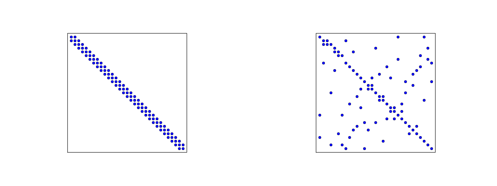 #
#
#
#
#
#
#
#
#
#
#
#
#
#
#
#
#
# Matrix sparsity pattern for left-to-right numbering (left) and random numbering (right) of nodes in P3 elements.
#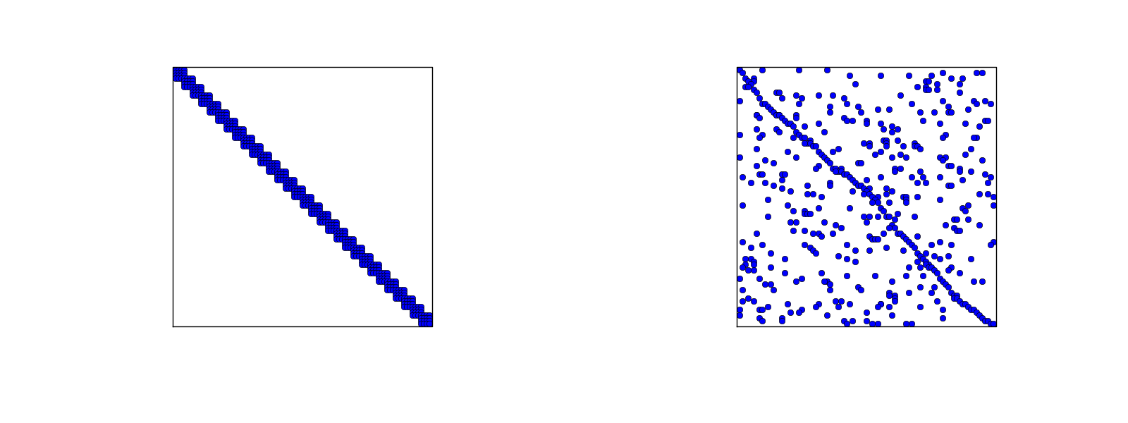 #
#
#
#
# The `scipy.sparse` library supports creation of sparse matrices
# and linear system solution.
#
# * `scipy.sparse.diags` for matrix defined via diagonals
#
# * `scipy.sparse.dok_matrix` for matrix incrementally defined via index pairs $(i,j)$
#
# The `dok_matrix` object is most convenient for finite element computations.
# This sparse matrix format is called DOK, which stands for Dictionary Of Keys:
# the implementation is basically a dictionary (hash) with the
# entry indices `(i,j)` as keys.
#
# Rather than declaring `A = np.zeros((N_n, N_n))`, a DOK sparse
# matrix is created by
# In[3]:
#DO NOT RUN THIS CELL
import scipy.sparse
A = scipy.sparse.dok_matrix((N_n, N_n))
# When there is any need to set or add some matrix entry `i,j`, just do
# In[85]:
#DO NOT RUN THIS CELL
A[i,j] = entry
# or
A[i,j] += entry
# The indexing creates the matrix entry on the fly, and
# only the nonzero entries in the matrix will be stored.
#
# To solve a system with right-hand side `b` (one-dimensional `numpy`
# array) with a sparse coefficient matrix `A`, we must use some kind of
# a sparse linear system solver. The safest choice is a method based on
# sparse Gaussian elimination. One high-quality package for
# this purpose if [UMFPACK](https://en.wikipedia.org/wiki/UMFPACK).
# It is interfaced from SciPy by
# In[86]:
#DO NOT RUN THIS CELL
import scipy.sparse.linalg
c = scipy.sparse.linalg.spsolve(A.tocsr(), b, use_umfpack=True)
# The call `A.tocsr()` is not strictly needed (a warning is issued
# otherwise), but ensures that the solution algorithm can efficiently
# work with a copy of the sparse matrix in *Compressed Sparse Row* (CSR) format.
#
# An advantage of the `scipy.sparse.diags` matrix over the DOK format is
# that the former allows vectorized assignment to the matrix.
# Vectorization is possible for approximation problems when all elements
# are of the same type. However, when solving differential equations,
# vectorization may be more difficult in particular because of boundary conditions.
# It also appears that the DOK sparse matrix format available in the `scipy.sparse` package is fast
# enough even for big 1D problems on today's laptops, so the need for
# improving efficiency occurs only in 2D and 3D problems, but then the
# complexity of the mesh favors the DOK format.
#
#
#
#
#
#
# # A generalized element concept
#
#
#
# So far, finite element computing has employed the `nodes` and
# `element` lists together with the definition of the basis functions
# in the reference element. Suppose we want to introduce a piecewise
# constant approximation with one basis function ${\tilde{\varphi}}_0(x)=1$ in
# the reference element, corresponding to a ${\varphi}_i(x)$ function that
# is 1 on element number $i$ and zero on all other elements.
# Although we could associate the function value
# with a node in the middle of the elements, there are no nodes at the
# ends, and the previous code snippets will not work because we
# cannot find the element boundaries from the `nodes` list.
#
# In order to get a richer space of finite element approximations, we need
# to revise the simple node and element concept presented so far and
# introduce a more powerful terminology. Much literature employs the
# definition of node and element introduced in the previous sections
# so it is important have this knowledge, besides being a good pedagogical
# background for understanding the extended element concept in the following.
#
# ## Cells, vertices, and degrees of freedom
#
#
#
# We now introduce *cells* as the subdomains $\Omega^{(e)}$ previously
# referred to as elements. The cell boundaries are uniquely defined in terms of *vertices*.
# This applies to cells in both 1D and higher dimensions.
# We also define a set of *degrees of freedom* (dof), which are
# the quantities we aim to compute. The most common type of degree
# of freedom is the value of the unknown function $u$ at some point.
# (For example, we can introduce nodes as before and say the degrees of
# freedom are the values of $u$ at the nodes.) The basis functions are
# constructed so that they equal unity for one particular degree of
# freedom and zero for the rest. This property ensures that when
# we evaluate $u=\sum_j c_j{\varphi}_j$ for degree of freedom number $i$,
# we get $u=c_i$. Integrals are performed over cells, usually by
# mapping the cell of interest to a *reference cell*.
#
#
# With the concepts of cells, vertices, and degrees of freedom we
# increase the decoupling of the geometry (cell, vertices) from the
# space of basis functions. We will associate different
# sets of basis functions with a cell. In 1D, all cells are intervals,
# while in 2D we can have cells that are triangles with straight sides,
# or any polygon, or in fact any two-dimensional geometry. Triangles and
# quadrilaterals are most common, though. The popular cell types in 3D
# are tetrahedra and hexahedra.
#
# ## Extended finite element concept
#
#
#
# The concept of a *finite element* is now
#
# * a *reference cell* in a local reference coordinate system;
#
# * a set of *basis functions* ${\tilde{\varphi}}_i$ defined on the cell;
#
# * a set of *degrees of freedom* that uniquely determine how basis functions
# from different elements are glued together across element interfaces.
# A common technique is to choose
# the basis functions such that ${\tilde{\varphi}}_i=1$ for degree of freedom
# number $i$ that is associated with nodal point
# $x_i$ and ${\tilde{\varphi}}_i=0$ for all other degrees of freedom. This
# technique ensures the desired continuity;
#
# * a mapping between local and global degree of freedom numbers,
# here called the *dof map*;
#
# * a geometric *mapping* of the reference cell onto the cell in the physical
# domain.
#
# There must be a geometric description of a cell. This is trivial in 1D
# since the cell is an interval and is described by the interval limits,
# here called vertices. If the cell is $\Omega^{(e)}=[x_L,x_R]$,
# vertex 0 is $x_L$ and vertex 1 is $x_R$. The reference cell in 1D
# is $[-1,1]$ in the reference coordinate system $X$.
#
#
# The expansion of $u$ over one cell is often used:
#
#
#
# $$
# \begin{equation}
# u(x) = \tilde u(X) = \sum_{r} c_r{\tilde{\varphi}}_r(X),\quad x\in\Omega^{(e)},\
# X\in [-1,1],
# \label{_auto52} \tag{108}
# \end{equation}
# $$
# where the sum is taken over the numbers of the degrees of freedom and
# $c_r$ is the value of $u$ for degree of freedom number $r$.
#
# Our previous P1, P2, etc., elements are defined by introducing $d+1$
# equally spaced nodes in the reference cell, a polynomial space (P$d$) containing
# a complete set of polynomials of order
# $d$, and saying that the degrees
# of freedom are the $d+1$ function values at these nodes. The basis
# functions must be 1 at one node and 0 at the others, and the Lagrange
# polynomials have exactly this property. The nodes can be numbered
# from left to right with associated degrees of freedom that are
# numbered in the same way. The degree of freedom mapping becomes what
# was previously represented by the `elements` lists. The cell mapping
# is the same affine mapping ([78](#fem:approx:fe:affine:mapping)) as
# before.
#
# **Notice.**
#
# The extended finite element concept introduced above is quite general and
# has served as a successful recipe for implementing many finite element frameworks
# and for developing the theory behind. Here, we have seen several different examples
# but the exposition is most focused on 1D examples and the diversity is limited
# as many of the different methods in 2D and 3D collapse to the same method in 1D.
# The curious reader is advised to for instance look into the numerous
# examples of finite elements implemented in FEniCS to gain insight into the variety of methods that exists.
#
#
#
#
#
# ## Implementation
#
#
#
# Implementationwise,
#
# * we replace `nodes` by `vertices`;
#
# * we introduce `cells` such that `cell[e][r]` gives the mapping
# from local vertex `r` in cell `e` to the global vertex number
# in `vertices`;
#
# * we replace `elements` by `dof_map` (the contents are the same
# for P$d$ elements).
#
# Consider the example from the section [Elements and nodes](#fem:approx:fe:def:elements:nodes) where $\Omega =[0,1]$ is divided
# into two cells, $\Omega^{(0)}=[0,0.4]$ and $\Omega^{(1)}=[0.4,1]$, as
# depicted in [Figure](#fem:approx:fe:def:elements:nodes:fig:P2). The
# vertices are $[0,0.4,1]$. Local vertex 0 and 1 are $0$ and $0.4$ in
# cell 0 and $0.4$ and $1$ in cell 1. A P2 element means that the
# degrees of freedom are the value of $u$ at three equally spaced points
# (nodes) in each cell. The data structures become
# In[4]:
vertices = [0, 0.4, 1]
cells = [[0, 1], [1, 2]]
dof_map = [[0, 1, 2], [2, 3, 4]]
# If we approximate $f$ by piecewise constants, known as
# P0 elements, we simply
# introduce one point or node in an element, preferably $X=0$,
# and define one degree of freedom, which is the function value
# at this node. Moreover, we set ${\tilde{\varphi}}_0(X)=1$.
# The `cells` and `vertices` arrays remain the same, but
# `dof_map` is altered:
# In[5]:
dof_map = [[0], [1]]
# We use the `cells` and `vertices` lists to retrieve information
# on the geometry of a cell, while `dof_map` is the
# $q(e,r)$ mapping introduced earlier in the
# assembly of element matrices and vectors.
# For example, the `Omega_e` variable (representing the cell interval)
# in previous code snippets must now be computed as
# In[ ]:
#DO NOT RUN THIS CELL
Omega_e = [vertices[cells[e][0]], vertices[cells[e][1]]]
# The assembly is done by
# In[ ]:
#DO NOT RUN THIS CELL
A[dof_map[e][r], dof_map[e][s]] += A_e[r,s]
b[dof_map[e][r]] += b_e[r]
# We will hereafter drop the `nodes` and `elements` arrays
# and work exclusively with `cells`, `vertices`, and `dof_map`.
# The module `fe_approx1D_numint.py` now replaces the module
# `fe_approx1D` and offers similar functions that work with
# the new concepts:
# In[7]:
from src.fe_approx1D_numint import *
x = sym.Symbol('x')
f = x*(1 - x)
N_e = 10
vertices, cells, dof_map = mesh_uniform(N_e, d=3, Omega=[0,1])
phi = [basis(len(dof_map[e])-1) for e in range(N_e)]
A, b = assemble(vertices, cells, dof_map, phi, f, False)
c = np.linalg.solve(A, b)
# Make very fine mesh and sample u(x) on this mesh for plotting
x_u, u = u_glob(c, vertices, cells, dof_map,
resolution_per_element=51)
plt.plot(x_u, u)
# These steps are offered in the `approximate` function, which we here
# apply to see how well four P0 elements (piecewise constants)
# can approximate a parabola:
# In[8]:
from src.fe_approx1D_numint import *
x=sym.Symbol("x")
for N_e in 4, 8:
approximate(x*(1-x), d=0, N_e=N_e, Omega=[0,1])
# [Figure](#fem:approx:fe:element:impl:fig:P0:x2) shows the result.
#
#
#
#
#
#
#
#
#
#
#
# The `scipy.sparse` library supports creation of sparse matrices
# and linear system solution.
#
# * `scipy.sparse.diags` for matrix defined via diagonals
#
# * `scipy.sparse.dok_matrix` for matrix incrementally defined via index pairs $(i,j)$
#
# The `dok_matrix` object is most convenient for finite element computations.
# This sparse matrix format is called DOK, which stands for Dictionary Of Keys:
# the implementation is basically a dictionary (hash) with the
# entry indices `(i,j)` as keys.
#
# Rather than declaring `A = np.zeros((N_n, N_n))`, a DOK sparse
# matrix is created by
# In[3]:
#DO NOT RUN THIS CELL
import scipy.sparse
A = scipy.sparse.dok_matrix((N_n, N_n))
# When there is any need to set or add some matrix entry `i,j`, just do
# In[85]:
#DO NOT RUN THIS CELL
A[i,j] = entry
# or
A[i,j] += entry
# The indexing creates the matrix entry on the fly, and
# only the nonzero entries in the matrix will be stored.
#
# To solve a system with right-hand side `b` (one-dimensional `numpy`
# array) with a sparse coefficient matrix `A`, we must use some kind of
# a sparse linear system solver. The safest choice is a method based on
# sparse Gaussian elimination. One high-quality package for
# this purpose if [UMFPACK](https://en.wikipedia.org/wiki/UMFPACK).
# It is interfaced from SciPy by
# In[86]:
#DO NOT RUN THIS CELL
import scipy.sparse.linalg
c = scipy.sparse.linalg.spsolve(A.tocsr(), b, use_umfpack=True)
# The call `A.tocsr()` is not strictly needed (a warning is issued
# otherwise), but ensures that the solution algorithm can efficiently
# work with a copy of the sparse matrix in *Compressed Sparse Row* (CSR) format.
#
# An advantage of the `scipy.sparse.diags` matrix over the DOK format is
# that the former allows vectorized assignment to the matrix.
# Vectorization is possible for approximation problems when all elements
# are of the same type. However, when solving differential equations,
# vectorization may be more difficult in particular because of boundary conditions.
# It also appears that the DOK sparse matrix format available in the `scipy.sparse` package is fast
# enough even for big 1D problems on today's laptops, so the need for
# improving efficiency occurs only in 2D and 3D problems, but then the
# complexity of the mesh favors the DOK format.
#
#
#
#
#
#
# # A generalized element concept
#
#
#
# So far, finite element computing has employed the `nodes` and
# `element` lists together with the definition of the basis functions
# in the reference element. Suppose we want to introduce a piecewise
# constant approximation with one basis function ${\tilde{\varphi}}_0(x)=1$ in
# the reference element, corresponding to a ${\varphi}_i(x)$ function that
# is 1 on element number $i$ and zero on all other elements.
# Although we could associate the function value
# with a node in the middle of the elements, there are no nodes at the
# ends, and the previous code snippets will not work because we
# cannot find the element boundaries from the `nodes` list.
#
# In order to get a richer space of finite element approximations, we need
# to revise the simple node and element concept presented so far and
# introduce a more powerful terminology. Much literature employs the
# definition of node and element introduced in the previous sections
# so it is important have this knowledge, besides being a good pedagogical
# background for understanding the extended element concept in the following.
#
# ## Cells, vertices, and degrees of freedom
#
#
#
# We now introduce *cells* as the subdomains $\Omega^{(e)}$ previously
# referred to as elements. The cell boundaries are uniquely defined in terms of *vertices*.
# This applies to cells in both 1D and higher dimensions.
# We also define a set of *degrees of freedom* (dof), which are
# the quantities we aim to compute. The most common type of degree
# of freedom is the value of the unknown function $u$ at some point.
# (For example, we can introduce nodes as before and say the degrees of
# freedom are the values of $u$ at the nodes.) The basis functions are
# constructed so that they equal unity for one particular degree of
# freedom and zero for the rest. This property ensures that when
# we evaluate $u=\sum_j c_j{\varphi}_j$ for degree of freedom number $i$,
# we get $u=c_i$. Integrals are performed over cells, usually by
# mapping the cell of interest to a *reference cell*.
#
#
# With the concepts of cells, vertices, and degrees of freedom we
# increase the decoupling of the geometry (cell, vertices) from the
# space of basis functions. We will associate different
# sets of basis functions with a cell. In 1D, all cells are intervals,
# while in 2D we can have cells that are triangles with straight sides,
# or any polygon, or in fact any two-dimensional geometry. Triangles and
# quadrilaterals are most common, though. The popular cell types in 3D
# are tetrahedra and hexahedra.
#
# ## Extended finite element concept
#
#
#
# The concept of a *finite element* is now
#
# * a *reference cell* in a local reference coordinate system;
#
# * a set of *basis functions* ${\tilde{\varphi}}_i$ defined on the cell;
#
# * a set of *degrees of freedom* that uniquely determine how basis functions
# from different elements are glued together across element interfaces.
# A common technique is to choose
# the basis functions such that ${\tilde{\varphi}}_i=1$ for degree of freedom
# number $i$ that is associated with nodal point
# $x_i$ and ${\tilde{\varphi}}_i=0$ for all other degrees of freedom. This
# technique ensures the desired continuity;
#
# * a mapping between local and global degree of freedom numbers,
# here called the *dof map*;
#
# * a geometric *mapping* of the reference cell onto the cell in the physical
# domain.
#
# There must be a geometric description of a cell. This is trivial in 1D
# since the cell is an interval and is described by the interval limits,
# here called vertices. If the cell is $\Omega^{(e)}=[x_L,x_R]$,
# vertex 0 is $x_L$ and vertex 1 is $x_R$. The reference cell in 1D
# is $[-1,1]$ in the reference coordinate system $X$.
#
#
# The expansion of $u$ over one cell is often used:
#
#
#
# $$
# \begin{equation}
# u(x) = \tilde u(X) = \sum_{r} c_r{\tilde{\varphi}}_r(X),\quad x\in\Omega^{(e)},\
# X\in [-1,1],
# \label{_auto52} \tag{108}
# \end{equation}
# $$
# where the sum is taken over the numbers of the degrees of freedom and
# $c_r$ is the value of $u$ for degree of freedom number $r$.
#
# Our previous P1, P2, etc., elements are defined by introducing $d+1$
# equally spaced nodes in the reference cell, a polynomial space (P$d$) containing
# a complete set of polynomials of order
# $d$, and saying that the degrees
# of freedom are the $d+1$ function values at these nodes. The basis
# functions must be 1 at one node and 0 at the others, and the Lagrange
# polynomials have exactly this property. The nodes can be numbered
# from left to right with associated degrees of freedom that are
# numbered in the same way. The degree of freedom mapping becomes what
# was previously represented by the `elements` lists. The cell mapping
# is the same affine mapping ([78](#fem:approx:fe:affine:mapping)) as
# before.
#
# **Notice.**
#
# The extended finite element concept introduced above is quite general and
# has served as a successful recipe for implementing many finite element frameworks
# and for developing the theory behind. Here, we have seen several different examples
# but the exposition is most focused on 1D examples and the diversity is limited
# as many of the different methods in 2D and 3D collapse to the same method in 1D.
# The curious reader is advised to for instance look into the numerous
# examples of finite elements implemented in FEniCS to gain insight into the variety of methods that exists.
#
#
#
#
#
# ## Implementation
#
#
#
# Implementationwise,
#
# * we replace `nodes` by `vertices`;
#
# * we introduce `cells` such that `cell[e][r]` gives the mapping
# from local vertex `r` in cell `e` to the global vertex number
# in `vertices`;
#
# * we replace `elements` by `dof_map` (the contents are the same
# for P$d$ elements).
#
# Consider the example from the section [Elements and nodes](#fem:approx:fe:def:elements:nodes) where $\Omega =[0,1]$ is divided
# into two cells, $\Omega^{(0)}=[0,0.4]$ and $\Omega^{(1)}=[0.4,1]$, as
# depicted in [Figure](#fem:approx:fe:def:elements:nodes:fig:P2). The
# vertices are $[0,0.4,1]$. Local vertex 0 and 1 are $0$ and $0.4$ in
# cell 0 and $0.4$ and $1$ in cell 1. A P2 element means that the
# degrees of freedom are the value of $u$ at three equally spaced points
# (nodes) in each cell. The data structures become
# In[4]:
vertices = [0, 0.4, 1]
cells = [[0, 1], [1, 2]]
dof_map = [[0, 1, 2], [2, 3, 4]]
# If we approximate $f$ by piecewise constants, known as
# P0 elements, we simply
# introduce one point or node in an element, preferably $X=0$,
# and define one degree of freedom, which is the function value
# at this node. Moreover, we set ${\tilde{\varphi}}_0(X)=1$.
# The `cells` and `vertices` arrays remain the same, but
# `dof_map` is altered:
# In[5]:
dof_map = [[0], [1]]
# We use the `cells` and `vertices` lists to retrieve information
# on the geometry of a cell, while `dof_map` is the
# $q(e,r)$ mapping introduced earlier in the
# assembly of element matrices and vectors.
# For example, the `Omega_e` variable (representing the cell interval)
# in previous code snippets must now be computed as
# In[ ]:
#DO NOT RUN THIS CELL
Omega_e = [vertices[cells[e][0]], vertices[cells[e][1]]]
# The assembly is done by
# In[ ]:
#DO NOT RUN THIS CELL
A[dof_map[e][r], dof_map[e][s]] += A_e[r,s]
b[dof_map[e][r]] += b_e[r]
# We will hereafter drop the `nodes` and `elements` arrays
# and work exclusively with `cells`, `vertices`, and `dof_map`.
# The module `fe_approx1D_numint.py` now replaces the module
# `fe_approx1D` and offers similar functions that work with
# the new concepts:
# In[7]:
from src.fe_approx1D_numint import *
x = sym.Symbol('x')
f = x*(1 - x)
N_e = 10
vertices, cells, dof_map = mesh_uniform(N_e, d=3, Omega=[0,1])
phi = [basis(len(dof_map[e])-1) for e in range(N_e)]
A, b = assemble(vertices, cells, dof_map, phi, f, False)
c = np.linalg.solve(A, b)
# Make very fine mesh and sample u(x) on this mesh for plotting
x_u, u = u_glob(c, vertices, cells, dof_map,
resolution_per_element=51)
plt.plot(x_u, u)
# These steps are offered in the `approximate` function, which we here
# apply to see how well four P0 elements (piecewise constants)
# can approximate a parabola:
# In[8]:
from src.fe_approx1D_numint import *
x=sym.Symbol("x")
for N_e in 4, 8:
approximate(x*(1-x), d=0, N_e=N_e, Omega=[0,1])
# [Figure](#fem:approx:fe:element:impl:fig:P0:x2) shows the result.
#
#
#
#
#
#
# Approximation of a parabola by 4 (left) and 8 (right) P0 elements.
# #
#
#
#
#
# ## Computing the error of the approximation
#
#
# So far we have focused on computing the coefficients $c_j$ in the
# approximation $u(x)=\sum_jc_j{\varphi}_j$ as well as on plotting $u$ and
# $f$ for visual comparison. A more quantitative comparison needs to
# investigate the error $e(x)=f(x)-u(x)$. We mostly want a single number to
# reflect the error and use a norm for this purpose, usually the $L^2$ norm
# $$
# ||e||_{L^2} = \left(\int_{\Omega} e^2 {\, \mathrm{d}x}\right)^{1/2}{\thinspace .}
# $$
# Since the finite element approximation is defined for all $x\in\Omega$,
# and we are interested in how $u(x)$ deviates from $f(x)$ through all
# the elements,
# we can either integrate analytically or use an accurate numerical
# approximation. The latter is more convenient as it is a generally
# feasible and simple approach. The idea is to sample $e(x)$
# at a large number of points in each element. The function `u_glob`
# in the `fe_approx1D_numint` module does this for $u(x)$ and returns
# an array `x` with coordinates and an array `u` with the $u$ values:
# In[ ]:
#DO NOT RUN THIS CELL
x, u = u_glob(c, vertices, cells, dof_map,
resolution_per_element=101)
e = f(x) - u
# Let us use the Trapezoidal method to approximate the integral. Because
# different elements may have different lengths, the `x` array may have
# a non-uniformly distributed set of coordinates. Also, the `u_glob`
# function works in an element by element fashion such that coordinates
# at the boundaries between elements appear twice. We therefore need
# to use a "raw" version of the Trapezoidal rule where we just add up
# all the trapezoids:
# $$
# \int_\Omega g(x) {\, \mathrm{d}x} \approx \sum_{j=0}^{n-1} \frac{1}{2}(g(x_j) +
# g(x_{j+1}))(x_{j+1}-x_j),
# $$
# if $x_0,\ldots,x_n$ are all the coordinates in `x`. In
# vectorized Python code,
# In[94]:
#DO NOT RUN THIS CELL
g_x = g(x)
integral = 0.5*np.sum((g_x[:-1] + g_x[1:])*(x[1:] - x[:-1]))
# Computing the $L^2$ norm of the error, here named `E`, is now achieved by
# In[95]:
#DO NOT RUN THIS CELL
e2 = e**2
E = np.sqrt(0.5*np.sum((e2[:-1] + e2[1:])*(x[1:] - x[:-1]))
#
# # Finite elements in 2D and 3D
#
# Finite element approximation is particularly powerful in 2D and 3D because
# the method can handle a geometrically complex domain $\Omega$ with ease.
# The principal idea is, as in 1D, to divide the domain into cells
# and use polynomials for approximating a function over a cell.
# Two popular cell shapes are triangles and quadrilaterals.
# It is common to denote finite elements on triangles and tetrahedrons as P while
# elements defined in terms of quadrilaterals and boxes are denoted by Q.
# Figures [fem:approx:fe:2D:fig:rectP1](#fem:approx:fe:2D:fig:rectP1), [fem:approx:fe:2D:fig:circP1](#fem:approx:fe:2D:fig:circP1),
# and [fem:approx:fe:2D:fig:rectQ1](#fem:approx:fe:2D:fig:rectQ1) provide examples. P1 elements
# means linear functions ($a_0 + a_1x + a_2y$) over triangles, while Q1 elements
# have bilinear functions ($a_0 + a_1x + a_2y + a_3xy$) over rectangular cells.
# Higher-order elements can easily be defined.
#
#
#
#
#
#
#
#
#
#
#
#
# ## Computing the error of the approximation
#
#
# So far we have focused on computing the coefficients $c_j$ in the
# approximation $u(x)=\sum_jc_j{\varphi}_j$ as well as on plotting $u$ and
# $f$ for visual comparison. A more quantitative comparison needs to
# investigate the error $e(x)=f(x)-u(x)$. We mostly want a single number to
# reflect the error and use a norm for this purpose, usually the $L^2$ norm
# $$
# ||e||_{L^2} = \left(\int_{\Omega} e^2 {\, \mathrm{d}x}\right)^{1/2}{\thinspace .}
# $$
# Since the finite element approximation is defined for all $x\in\Omega$,
# and we are interested in how $u(x)$ deviates from $f(x)$ through all
# the elements,
# we can either integrate analytically or use an accurate numerical
# approximation. The latter is more convenient as it is a generally
# feasible and simple approach. The idea is to sample $e(x)$
# at a large number of points in each element. The function `u_glob`
# in the `fe_approx1D_numint` module does this for $u(x)$ and returns
# an array `x` with coordinates and an array `u` with the $u$ values:
# In[ ]:
#DO NOT RUN THIS CELL
x, u = u_glob(c, vertices, cells, dof_map,
resolution_per_element=101)
e = f(x) - u
# Let us use the Trapezoidal method to approximate the integral. Because
# different elements may have different lengths, the `x` array may have
# a non-uniformly distributed set of coordinates. Also, the `u_glob`
# function works in an element by element fashion such that coordinates
# at the boundaries between elements appear twice. We therefore need
# to use a "raw" version of the Trapezoidal rule where we just add up
# all the trapezoids:
# $$
# \int_\Omega g(x) {\, \mathrm{d}x} \approx \sum_{j=0}^{n-1} \frac{1}{2}(g(x_j) +
# g(x_{j+1}))(x_{j+1}-x_j),
# $$
# if $x_0,\ldots,x_n$ are all the coordinates in `x`. In
# vectorized Python code,
# In[94]:
#DO NOT RUN THIS CELL
g_x = g(x)
integral = 0.5*np.sum((g_x[:-1] + g_x[1:])*(x[1:] - x[:-1]))
# Computing the $L^2$ norm of the error, here named `E`, is now achieved by
# In[95]:
#DO NOT RUN THIS CELL
e2 = e**2
E = np.sqrt(0.5*np.sum((e2[:-1] + e2[1:])*(x[1:] - x[:-1]))
#
# # Finite elements in 2D and 3D
#
# Finite element approximation is particularly powerful in 2D and 3D because
# the method can handle a geometrically complex domain $\Omega$ with ease.
# The principal idea is, as in 1D, to divide the domain into cells
# and use polynomials for approximating a function over a cell.
# Two popular cell shapes are triangles and quadrilaterals.
# It is common to denote finite elements on triangles and tetrahedrons as P while
# elements defined in terms of quadrilaterals and boxes are denoted by Q.
# Figures [fem:approx:fe:2D:fig:rectP1](#fem:approx:fe:2D:fig:rectP1), [fem:approx:fe:2D:fig:circP1](#fem:approx:fe:2D:fig:circP1),
# and [fem:approx:fe:2D:fig:rectQ1](#fem:approx:fe:2D:fig:rectQ1) provide examples. P1 elements
# means linear functions ($a_0 + a_1x + a_2y$) over triangles, while Q1 elements
# have bilinear functions ($a_0 + a_1x + a_2y + a_3xy$) over rectangular cells.
# Higher-order elements can easily be defined.
#
#
#
#
#
#
# Example on 2D P1 elements.
#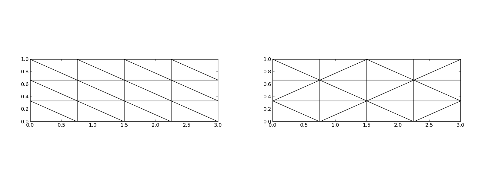 #
#
#
#
#
#
#
#
#
#
#
#
#
#
#
#
#
# Example on 2D P1 elements in a deformed geometry.
# #
#
#
#
#
#
#
#
#
#
#
#
#
#
#
#
#
# Example on 2D Q1 elements.
# #
#
#
#
#
# ## Basis functions over triangles in the physical domain
#
# Cells with triangular shape will be in main focus here. With the P1
# triangular element, $u$ is a linear function over each cell, as
# depicted in [Figure](#fem:approx:fe:2D:fig:femfunc), with
# discontinuous derivatives at the cell boundaries.
#
#
#
#
#
#
#
#
#
#
#
# ## Basis functions over triangles in the physical domain
#
# Cells with triangular shape will be in main focus here. With the P1
# triangular element, $u$ is a linear function over each cell, as
# depicted in [Figure](#fem:approx:fe:2D:fig:femfunc), with
# discontinuous derivatives at the cell boundaries.
#
#
#
#
#
# Example on scalar function defined in terms of piecewise linear 2D functions defined on triangles.
#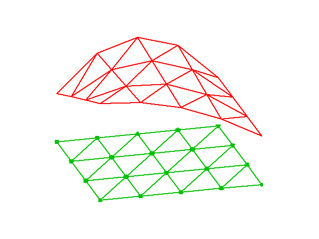 #
#
#
#
# We give the vertices of the cells global and local numbers as in 1D.
# The degrees of freedom in the P1 element are the function values at
# a set of nodes, which are the three vertices.
# The basis function ${\varphi}_i(x,y)$ is then 1 at the vertex with global vertex
# number $i$ and zero at all other vertices.
# On an element, the three degrees of freedom uniquely determine
# the linear basis functions in that element, as usual.
# The global
# ${\varphi}_i(x,y)$ function is then a combination of the linear functions
# (planar surfaces)
# over all the neighboring cells
# that have vertex number $i$ in common. [Figure](#fem:approx:fe:2D:fig:basphi)
# tries to illustrate the shape of such a "pyramid"-like function.
#
#
#
#
#
#
#
#
#
#
# We give the vertices of the cells global and local numbers as in 1D.
# The degrees of freedom in the P1 element are the function values at
# a set of nodes, which are the three vertices.
# The basis function ${\varphi}_i(x,y)$ is then 1 at the vertex with global vertex
# number $i$ and zero at all other vertices.
# On an element, the three degrees of freedom uniquely determine
# the linear basis functions in that element, as usual.
# The global
# ${\varphi}_i(x,y)$ function is then a combination of the linear functions
# (planar surfaces)
# over all the neighboring cells
# that have vertex number $i$ in common. [Figure](#fem:approx:fe:2D:fig:basphi)
# tries to illustrate the shape of such a "pyramid"-like function.
#
#
#
#
#
# Example on a piecewise linear 2D basis function over a patch of triangles.
#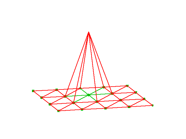 #
#
#
#
# ### Element matrices and vectors
#
# As in 1D, we split the integral over $\Omega$ into a sum of integrals
# over cells. Also as in 1D, ${\varphi}_i$ overlaps ${\varphi}_j$
# (i.e., ${\varphi}_i{\varphi}_j\neq 0$) if and only if
# $i$ and $j$ are vertices in the same cell. Therefore, the integral
# of ${\varphi}_i{\varphi}_j$ over an element is nonzero only when $i$ and $j$
# run over the vertex numbers in the element. These nonzero contributions
# to the coefficient matrix are, as in 1D, collected in an element matrix.
# The size of the element matrix becomes $3\times 3$ since there are
# three degrees of freedom
# that $i$ and $j$ run over. Again, as in 1D, we number the
# local vertices in a cell, starting at 0, and add the entries in
# the element matrix into the global system matrix, exactly as in 1D.
# All the details and code appear below.
#
#
#
# ## Basis functions over triangles in the reference cell
#
# As in 1D, we can define the basis functions and the degrees of freedom
# in a reference cell and then use a mapping from the reference coordinate
# system to the physical coordinate system.
# We also need a mapping of local degrees of freedom numbers to global degrees
# of freedom numbers.
#
#
# The reference cell in an $(X,Y)$ coordinate system has vertices
# $(0,0)$, $(1,0)$, and $(0,1)$, corresponding to local vertex numbers
# 0, 1, and 2, respectively. The P1 element has linear functions
# ${\tilde{\varphi}}_r(X,Y)$ as basis functions, $r=0,1,2$.
# Since a linear function ${\tilde{\varphi}}_r(X,Y)$ in 2D is of
# the form $C_{r,0} + C_{r,1}X + C_{r,2}Y$, and hence has three
# parameters $C_{r,0}$, $C_{r,1}$, and $C_{r,2}$, we need three
# degrees of freedom. These are in general taken as the function values at a
# set of nodes. For the P1 element the set of nodes is the three vertices.
# [Figure](#fem:approx:fe:2D:fig:P12D) displays the geometry of the
# element and the location of the nodes.
#
#
#
#
#
#
#
#
#
#
# ### Element matrices and vectors
#
# As in 1D, we split the integral over $\Omega$ into a sum of integrals
# over cells. Also as in 1D, ${\varphi}_i$ overlaps ${\varphi}_j$
# (i.e., ${\varphi}_i{\varphi}_j\neq 0$) if and only if
# $i$ and $j$ are vertices in the same cell. Therefore, the integral
# of ${\varphi}_i{\varphi}_j$ over an element is nonzero only when $i$ and $j$
# run over the vertex numbers in the element. These nonzero contributions
# to the coefficient matrix are, as in 1D, collected in an element matrix.
# The size of the element matrix becomes $3\times 3$ since there are
# three degrees of freedom
# that $i$ and $j$ run over. Again, as in 1D, we number the
# local vertices in a cell, starting at 0, and add the entries in
# the element matrix into the global system matrix, exactly as in 1D.
# All the details and code appear below.
#
#
#
# ## Basis functions over triangles in the reference cell
#
# As in 1D, we can define the basis functions and the degrees of freedom
# in a reference cell and then use a mapping from the reference coordinate
# system to the physical coordinate system.
# We also need a mapping of local degrees of freedom numbers to global degrees
# of freedom numbers.
#
#
# The reference cell in an $(X,Y)$ coordinate system has vertices
# $(0,0)$, $(1,0)$, and $(0,1)$, corresponding to local vertex numbers
# 0, 1, and 2, respectively. The P1 element has linear functions
# ${\tilde{\varphi}}_r(X,Y)$ as basis functions, $r=0,1,2$.
# Since a linear function ${\tilde{\varphi}}_r(X,Y)$ in 2D is of
# the form $C_{r,0} + C_{r,1}X + C_{r,2}Y$, and hence has three
# parameters $C_{r,0}$, $C_{r,1}$, and $C_{r,2}$, we need three
# degrees of freedom. These are in general taken as the function values at a
# set of nodes. For the P1 element the set of nodes is the three vertices.
# [Figure](#fem:approx:fe:2D:fig:P12D) displays the geometry of the
# element and the location of the nodes.
#
#
#
#
#
# 2D P1 element.
#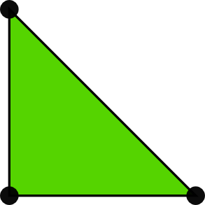 #
#
#
#
# Requiring ${\tilde{\varphi}}_r=1$ at node number $r$ and
# ${\tilde{\varphi}}_r=0$ at the two other nodes, gives three linear equations to
# determine $C_{r,0}$, $C_{r,1}$, and $C_{r,2}$. The result is
#
#
#
# $$
# \begin{equation}
# {\tilde{\varphi}}_0(X,Y) = 1 - X - Y,
# \label{_auto63} \tag{122}
# \end{equation}
# $$
#
#
#
# $$
# \begin{equation}
# {\tilde{\varphi}}_1(X,Y) = X,
# \label{_auto64} \tag{123}
# \end{equation}
# $$
#
#
#
# $$
# \begin{equation}
# {\tilde{\varphi}}_2(X,Y) = Y
# \label{_auto65} \tag{124}
# \end{equation}
# $$
# Higher-order approximations are obtained by increasing the polynomial order,
# adding additional nodes, and letting the degrees of freedom be
# function values at the nodes. [Figure](#fem:approx:fe:2D:fig:P22D)
# shows the location of the six nodes in the P2 element.
#
#
#
#
#
#
#
#
#
#
# Requiring ${\tilde{\varphi}}_r=1$ at node number $r$ and
# ${\tilde{\varphi}}_r=0$ at the two other nodes, gives three linear equations to
# determine $C_{r,0}$, $C_{r,1}$, and $C_{r,2}$. The result is
#
#
#
# $$
# \begin{equation}
# {\tilde{\varphi}}_0(X,Y) = 1 - X - Y,
# \label{_auto63} \tag{122}
# \end{equation}
# $$
#
#
#
# $$
# \begin{equation}
# {\tilde{\varphi}}_1(X,Y) = X,
# \label{_auto64} \tag{123}
# \end{equation}
# $$
#
#
#
# $$
# \begin{equation}
# {\tilde{\varphi}}_2(X,Y) = Y
# \label{_auto65} \tag{124}
# \end{equation}
# $$
# Higher-order approximations are obtained by increasing the polynomial order,
# adding additional nodes, and letting the degrees of freedom be
# function values at the nodes. [Figure](#fem:approx:fe:2D:fig:P22D)
# shows the location of the six nodes in the P2 element.
#
#
#
#
#
# 2D P2 element.
#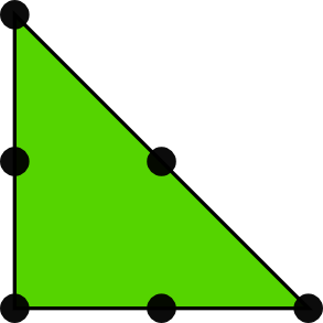 #
#
#
#
#
#
# A polynomial of degree $p$ in $X$ and $Y$ has $n_p=(p+1)(p+2)/2$ terms
# and hence needs $n_p$ nodes. The values at the nodes constitute $n_p$
# degrees of freedom. The location of the nodes for
# ${\tilde{\varphi}}_r$ up to degree 6 is displayed in [Figure](#fem:approx:fe:2D:fig:P162D).
#
#
#
#
#
#
#
#
#
#
#
#
# A polynomial of degree $p$ in $X$ and $Y$ has $n_p=(p+1)(p+2)/2$ terms
# and hence needs $n_p$ nodes. The values at the nodes constitute $n_p$
# degrees of freedom. The location of the nodes for
# ${\tilde{\varphi}}_r$ up to degree 6 is displayed in [Figure](#fem:approx:fe:2D:fig:P162D).
#
#
#
#
#
# 2D P1, P2, P3, P4, P5, and P6 elements.
# #
#
#
#
# The generalization to 3D is straightforward: the reference element is a
# [tetrahedron](http://en.wikipedia.org/wiki/Tetrahedron)
# with vertices $(0,0,0)$, $(1,0,0)$, $(0,1,0)$, and $(0,0,1)$
# in a $X,Y,Z$ reference coordinate system. The P1 element has its degrees
# of freedom as four nodes, which are the four vertices, see [Figure](#fem:approx:fe:2D:fig:P1:123D). The P2 element adds additional
# nodes along the edges of the cell, yielding a total of 10 nodes and
# degrees of freedom, see
# [Figure](#fem:approx:fe:2D:fig:P2:123D).
#
#
#
#
#
#
#
#
#
#
# The generalization to 3D is straightforward: the reference element is a
# [tetrahedron](http://en.wikipedia.org/wiki/Tetrahedron)
# with vertices $(0,0,0)$, $(1,0,0)$, $(0,1,0)$, and $(0,0,1)$
# in a $X,Y,Z$ reference coordinate system. The P1 element has its degrees
# of freedom as four nodes, which are the four vertices, see [Figure](#fem:approx:fe:2D:fig:P1:123D). The P2 element adds additional
# nodes along the edges of the cell, yielding a total of 10 nodes and
# degrees of freedom, see
# [Figure](#fem:approx:fe:2D:fig:P2:123D).
#
#
#
#
#
# P1 elements in 1D, 2D, and 3D.
# #
#
#
#
#
#
#
#
#
#
#
#
#
#
#
#
#
# P2 elements in 1D, 2D, and 3D.
#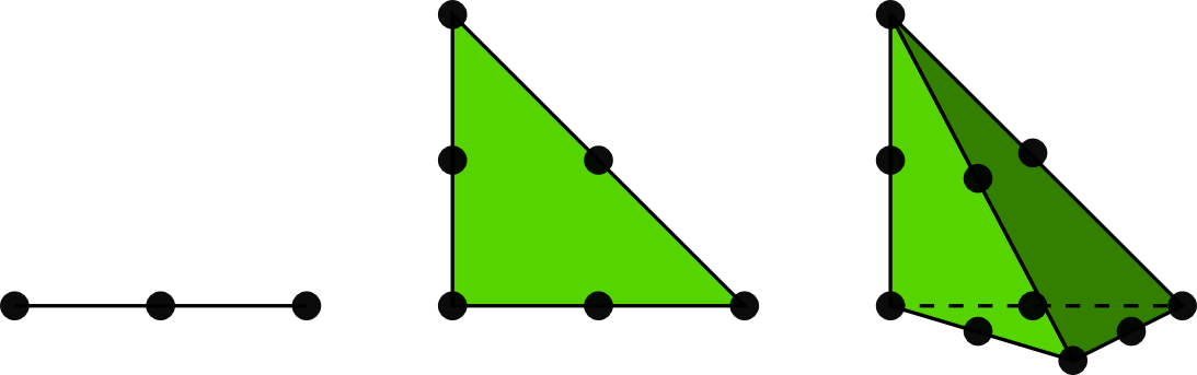 #
#
#
#
#
# The interval in 1D, the triangle in 2D, the tetrahedron in 3D, and
# its generalizations to higher space dimensions are known
# as *simplex* cells (the geometry) or *simplex* elements (the geometry,
# basis functions, degrees of freedom, etc.). The plural forms
# [simplices](http://en.wikipedia.org/wiki/Simplex) and
# simplexes are
# also much used shorter terms when referring to this type of cells or elements.
# The side of a simplex is called a *face*, while the tetrahedron also
# has *edges*.
#
#
# **Acknowledgment.**
# Figures [fem:approx:fe:2D:fig:P12D](#fem:approx:fe:2D:fig:P12D)-[fem:approx:fe:2D:fig:P2:123D](#fem:approx:fe:2D:fig:P2:123D)
# are created by Anders Logg and taken from the [FEniCS book](https://launchpad.net/fenics-book): *Automated Solution of Differential Equations by the Finite Element Method*, edited by A. Logg, K.-A. Mardal, and G. N. Wells, published
# by [Springer](http://goo.gl/lbyVMH), 2012.
#
#
#
# ## Affine mapping of the reference cell
#
# Let ${\tilde{\varphi}}_r^{(1)}$ denote the basis functions associated
# with the P1 element in 1D, 2D, or 3D, and let $\boldsymbol{x}_{q(e,r)}$ be
# the physical coordinates of local vertex number $r$ in cell $e$.
# Furthermore,
# let $\boldsymbol{X}$ be a point in the reference coordinate system corresponding
# to the point $\boldsymbol{x}$ in the physical coordinate system.
# The affine mapping of any $\boldsymbol{X}$ onto $\boldsymbol{x}$ is
# then defined by
#
#
#
# $$
# \begin{equation}
# \boldsymbol{x} = \sum_{r} {\tilde{\varphi}}_r^{(1)}(\boldsymbol{X})\boldsymbol{x}_{q(e,r)},
# \label{fem:approx:fe:affine:map} \tag{125}
# \end{equation}
# $$
# where $r$ runs over the local vertex numbers in the cell.
# The affine mapping essentially stretches, translates, and rotates
# the triangle. Straight or planar faces of the reference cell are
# therefore mapped onto
# straight or planar faces in the physical coordinate system. The mapping can
# be used for both P1 and higher-order elements, but note that the
# mapping itself always applies the P1 basis functions.
#
#
#
#
#
#
#
#
#
#
#
# The interval in 1D, the triangle in 2D, the tetrahedron in 3D, and
# its generalizations to higher space dimensions are known
# as *simplex* cells (the geometry) or *simplex* elements (the geometry,
# basis functions, degrees of freedom, etc.). The plural forms
# [simplices](http://en.wikipedia.org/wiki/Simplex) and
# simplexes are
# also much used shorter terms when referring to this type of cells or elements.
# The side of a simplex is called a *face*, while the tetrahedron also
# has *edges*.
#
#
# **Acknowledgment.**
# Figures [fem:approx:fe:2D:fig:P12D](#fem:approx:fe:2D:fig:P12D)-[fem:approx:fe:2D:fig:P2:123D](#fem:approx:fe:2D:fig:P2:123D)
# are created by Anders Logg and taken from the [FEniCS book](https://launchpad.net/fenics-book): *Automated Solution of Differential Equations by the Finite Element Method*, edited by A. Logg, K.-A. Mardal, and G. N. Wells, published
# by [Springer](http://goo.gl/lbyVMH), 2012.
#
#
#
# ## Affine mapping of the reference cell
#
# Let ${\tilde{\varphi}}_r^{(1)}$ denote the basis functions associated
# with the P1 element in 1D, 2D, or 3D, and let $\boldsymbol{x}_{q(e,r)}$ be
# the physical coordinates of local vertex number $r$ in cell $e$.
# Furthermore,
# let $\boldsymbol{X}$ be a point in the reference coordinate system corresponding
# to the point $\boldsymbol{x}$ in the physical coordinate system.
# The affine mapping of any $\boldsymbol{X}$ onto $\boldsymbol{x}$ is
# then defined by
#
#
#
# $$
# \begin{equation}
# \boldsymbol{x} = \sum_{r} {\tilde{\varphi}}_r^{(1)}(\boldsymbol{X})\boldsymbol{x}_{q(e,r)},
# \label{fem:approx:fe:affine:map} \tag{125}
# \end{equation}
# $$
# where $r$ runs over the local vertex numbers in the cell.
# The affine mapping essentially stretches, translates, and rotates
# the triangle. Straight or planar faces of the reference cell are
# therefore mapped onto
# straight or planar faces in the physical coordinate system. The mapping can
# be used for both P1 and higher-order elements, but note that the
# mapping itself always applies the P1 basis functions.
#
#
#
#
#
# Affine mapping of a P1 element.
#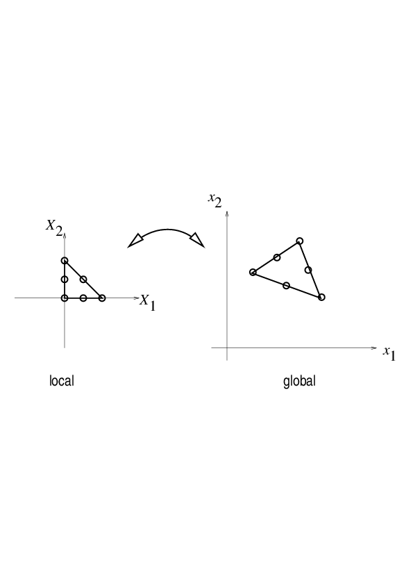 #
#
#
#
#
# ## Isoparametric mapping of the reference cell
#
#
# Instead of using the P1 basis functions in the mapping
# ([125](#fem:approx:fe:affine:map)),
# we may use the basis functions of the actual P$d$ element:
#
#
#
# $$
# \begin{equation}
# \boldsymbol{x} = \sum_{r} {\tilde{\varphi}}_r(\boldsymbol{X})\boldsymbol{x}_{q(e,r)},
# \label{fem:approx:fe:isop:map} \tag{126}
# \end{equation}
# $$
# where $r$ runs over all nodes, i.e., all points associated with the
# degrees of freedom. This is called an *isoparametric mapping*.
# For P1 elements it is identical to the affine mapping
# ([125](#fem:approx:fe:affine:map)), but for higher-order elements
# the mapping of the straight or planar faces of the reference cell will
# result in a *curved* face in the physical coordinate system.
# For example, when we use the basis functions of the triangular P2 element
# in 2D in ([126](#fem:approx:fe:isop:map)), the straight faces of the
# reference triangle are mapped onto curved faces of parabolic shape in
# the physical coordinate system, see [Figure](#fem:approx:fe:map:fig:2DP2).
#
#
#
#
#
#
#
#
#
#
#
# ## Isoparametric mapping of the reference cell
#
#
# Instead of using the P1 basis functions in the mapping
# ([125](#fem:approx:fe:affine:map)),
# we may use the basis functions of the actual P$d$ element:
#
#
#
# $$
# \begin{equation}
# \boldsymbol{x} = \sum_{r} {\tilde{\varphi}}_r(\boldsymbol{X})\boldsymbol{x}_{q(e,r)},
# \label{fem:approx:fe:isop:map} \tag{126}
# \end{equation}
# $$
# where $r$ runs over all nodes, i.e., all points associated with the
# degrees of freedom. This is called an *isoparametric mapping*.
# For P1 elements it is identical to the affine mapping
# ([125](#fem:approx:fe:affine:map)), but for higher-order elements
# the mapping of the straight or planar faces of the reference cell will
# result in a *curved* face in the physical coordinate system.
# For example, when we use the basis functions of the triangular P2 element
# in 2D in ([126](#fem:approx:fe:isop:map)), the straight faces of the
# reference triangle are mapped onto curved faces of parabolic shape in
# the physical coordinate system, see [Figure](#fem:approx:fe:map:fig:2DP2).
#
#
#
#
#
# Isoparametric mapping of a P2 element.
#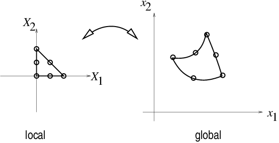 #
#
#
#
# From ([125](#fem:approx:fe:affine:map)) or
# ([126](#fem:approx:fe:isop:map)) it is easy to realize that the
# vertices are correctly mapped. Consider a vertex with local number $s$.
# Then ${\tilde{\varphi}}_s=1$ at this vertex and zero at the others.
# This means that only one term in the sum is nonzero and $\boldsymbol{x}=\boldsymbol{x}_{q(e,s)}$,
# which is the coordinate of this vertex in the global coordinate system.
#
#
# ## Computing integrals
#
# Let $\tilde\Omega^r$ denote the reference cell and $\Omega^{(e)}$
# the cell in the physical coordinate system. The transformation of
# the integral from the physical to the reference coordinate system reads
#
#
#
# $$
# \begin{equation}
# \int_{\Omega^{(e)}}{\varphi}_i (\boldsymbol{x}) {\varphi}_j (\boldsymbol{x}) {\, \mathrm{d}x} =
# \int_{\tilde\Omega^r} {\tilde{\varphi}}_i (\boldsymbol{X}) {\tilde{\varphi}}_j (\boldsymbol{X})
# \det J\, {\, \mathrm{d}X},
# \label{_auto66} \tag{127}
# \end{equation}
# $$
#
#
#
# $$
# \begin{equation}
# \int_{\Omega^{(e)}}{\varphi}_i (\boldsymbol{x}) f(\boldsymbol{x}) {\, \mathrm{d}x} =
# \int_{\tilde\Omega^r} {\tilde{\varphi}}_i (\boldsymbol{X}) f(\boldsymbol{x}(\boldsymbol{X})) \det J\, {\, \mathrm{d}X},
# \label{_auto67} \tag{128}
# \end{equation}
# $$
# where ${\, \mathrm{d}x}$ means the infinitesimal area element $dx dy$ in 2D and
# $dx dy dz$ in 3D, with a similar
# definition of ${\, \mathrm{d}X}$. The quantity $\det J$ is the determinant of the
# Jacobian of the mapping $\boldsymbol{x}(\boldsymbol{X})$. In 2D,
#
#
#
# $$
# \begin{equation}
# J = \left[\begin{array}{cc}
# \frac{\partial x}{\partial X} & \frac{\partial x}{\partial Y}\\
# \frac{\partial y}{\partial X} & \frac{\partial y}{\partial Y}
# \end{array}\right], \quad
# \det J = \frac{\partial x}{\partial X}\frac{\partial y}{\partial Y}
# - \frac{\partial x}{\partial Y}\frac{\partial y}{\partial X}
# {\thinspace .}
# \label{fem:approx:fe:2D:mapping:J:detJ} \tag{129}
# \end{equation}
# $$
# With the affine mapping
# ([125](#fem:approx:fe:affine:map)), $\det J=2\Delta$, where $\Delta$ is
# the area or volume of the cell in the physical coordinate system.
#
# **Remark.**
# Observe that finite elements in 2D and 3D build on the same
# *ideas* and *concepts* as in 1D, but there is simply much
# more to compute because the
# specific mathematical formulas in 2D and 3D are more complicated
# and the book-keeping with dof maps also gets more complicated.
# The manual work is tedious, lengthy, and error-prone
# so automation by the computer is a must.
#
#
#
#
#
#
#
#
#
#
#
#
#
#
#
#
#
#
#
#
#
#
#
#
# # Implementation
#
#
#
# Our previous programs for doing 1D approximation by finite element
# basis function had a focus on all the small details needed to compute
# the solution. When going to 2D and 3D, the basic algorithms are the
# same, but the amount of computational detail with basis functions,
# reference functions, mappings, numerical integration and so on,
# becomes overwhelming because of all the flexibility and choices of
# elements. For this purpose, we *must*, except in the simplest cases
# with P1 elements, use some well-developed, existing computer
# library.
# ## Example of approximation in 2D using FEniCS
#
#
# Here we shall use [FEniCS](http://fenicsproject.org), which
# is a free, open source finite element package for advanced computations. The
# package can be programmed in C++ or Python. How it works is best
# illustrated by an example.
#
# ### Mathematical problem
#
# We want to approximate the function $f(x)=2xy - x^2$ by P1 and P2 elements
# on $[0,2]\times[-1,1]$ using a division into $8\times 8$ squares, which are
# then divided into rectangles and then into triangles.
#
# ### The code
#
# Observe that the code employs the basic concepts from 1D, but is
# capable of using *any* element in FEniCS on *any* mesh in *any* number of
# space dimensions (!).
# In[96]:
from fenics import *
def approx(f, V):
"""Return Galerkin approximation to f in V."""
u = TrialFunction(V)
v = TestFunction(V)
a = u*v*dx
L = f*v*dx
u = Function(V)
solve(a == L, u)
return u
def problem():
f = Expression('2*x[0]*x[1] - pow(x[0], 2)', degree=2)
mesh = RectangleMesh(Point(0,-1), Point(2,1), 8, 8)
V1 = FunctionSpace(mesh, 'P', 1)
u1 = approx(f, V1)
u1.rename('u1', 'u1')
u1_error = errornorm(f, u1, 'L2')
u1_norm = norm(u1, 'L2')
V2 = FunctionSpace(mesh, 'P', 2)
u2 = approx(f, V2)
u2.rename('u2', 'u2')
u2_error = errornorm(f, u2, 'L2')
u2_norm = norm(u2, 'L2')
print(('L2 errors: e1=%g, e2=%g' % (u1_error, u2_error)))
print(('L2 norms: n1=%g, n2=%g' % (u1_norm, u2_norm)))
# Simple plotting
import matplotlib.pyplot as plt
plot(f, title='f', mesh=mesh)
plt.show()
plot(u1, title='u1')
plt.show()
plot(u2, title='u2')
plt.show()
if __name__ == '__main__':
problem()
# [Figure](#fem:approx:fenics:2D:fig1) shows the computed `u1`. The plots of
# `u2` and `f` are identical and therefore not shown.
# The plot shows that visually the approximation is quite close to
# `f`, but to quantify it more precisely we simply compute the
# error using the function `errornorm`. The output
# of errors becomes
# L2 errors: e1=0.01314, e2=4.93418e-15
# L2 norms: n1=4.46217, n2=4.46219
#
# Hence, the second order approximation `u2` is able to reproduce
# `f` up to floating point precision, whereas the first
# order approximation `u1` has an error of slightly more than $\frac{1}{3}$\%.
#
#
#
#
#
#
#
#
#
#
#
#
#
# From ([125](#fem:approx:fe:affine:map)) or
# ([126](#fem:approx:fe:isop:map)) it is easy to realize that the
# vertices are correctly mapped. Consider a vertex with local number $s$.
# Then ${\tilde{\varphi}}_s=1$ at this vertex and zero at the others.
# This means that only one term in the sum is nonzero and $\boldsymbol{x}=\boldsymbol{x}_{q(e,s)}$,
# which is the coordinate of this vertex in the global coordinate system.
#
#
# ## Computing integrals
#
# Let $\tilde\Omega^r$ denote the reference cell and $\Omega^{(e)}$
# the cell in the physical coordinate system. The transformation of
# the integral from the physical to the reference coordinate system reads
#
#
#
# $$
# \begin{equation}
# \int_{\Omega^{(e)}}{\varphi}_i (\boldsymbol{x}) {\varphi}_j (\boldsymbol{x}) {\, \mathrm{d}x} =
# \int_{\tilde\Omega^r} {\tilde{\varphi}}_i (\boldsymbol{X}) {\tilde{\varphi}}_j (\boldsymbol{X})
# \det J\, {\, \mathrm{d}X},
# \label{_auto66} \tag{127}
# \end{equation}
# $$
#
#
#
# $$
# \begin{equation}
# \int_{\Omega^{(e)}}{\varphi}_i (\boldsymbol{x}) f(\boldsymbol{x}) {\, \mathrm{d}x} =
# \int_{\tilde\Omega^r} {\tilde{\varphi}}_i (\boldsymbol{X}) f(\boldsymbol{x}(\boldsymbol{X})) \det J\, {\, \mathrm{d}X},
# \label{_auto67} \tag{128}
# \end{equation}
# $$
# where ${\, \mathrm{d}x}$ means the infinitesimal area element $dx dy$ in 2D and
# $dx dy dz$ in 3D, with a similar
# definition of ${\, \mathrm{d}X}$. The quantity $\det J$ is the determinant of the
# Jacobian of the mapping $\boldsymbol{x}(\boldsymbol{X})$. In 2D,
#
#
#
# $$
# \begin{equation}
# J = \left[\begin{array}{cc}
# \frac{\partial x}{\partial X} & \frac{\partial x}{\partial Y}\\
# \frac{\partial y}{\partial X} & \frac{\partial y}{\partial Y}
# \end{array}\right], \quad
# \det J = \frac{\partial x}{\partial X}\frac{\partial y}{\partial Y}
# - \frac{\partial x}{\partial Y}\frac{\partial y}{\partial X}
# {\thinspace .}
# \label{fem:approx:fe:2D:mapping:J:detJ} \tag{129}
# \end{equation}
# $$
# With the affine mapping
# ([125](#fem:approx:fe:affine:map)), $\det J=2\Delta$, where $\Delta$ is
# the area or volume of the cell in the physical coordinate system.
#
# **Remark.**
# Observe that finite elements in 2D and 3D build on the same
# *ideas* and *concepts* as in 1D, but there is simply much
# more to compute because the
# specific mathematical formulas in 2D and 3D are more complicated
# and the book-keeping with dof maps also gets more complicated.
# The manual work is tedious, lengthy, and error-prone
# so automation by the computer is a must.
#
#
#
#
#
#
#
#
#
#
#
#
#
#
#
#
#
#
#
#
#
#
#
#
# # Implementation
#
#
#
# Our previous programs for doing 1D approximation by finite element
# basis function had a focus on all the small details needed to compute
# the solution. When going to 2D and 3D, the basic algorithms are the
# same, but the amount of computational detail with basis functions,
# reference functions, mappings, numerical integration and so on,
# becomes overwhelming because of all the flexibility and choices of
# elements. For this purpose, we *must*, except in the simplest cases
# with P1 elements, use some well-developed, existing computer
# library.
# ## Example of approximation in 2D using FEniCS
#
#
# Here we shall use [FEniCS](http://fenicsproject.org), which
# is a free, open source finite element package for advanced computations. The
# package can be programmed in C++ or Python. How it works is best
# illustrated by an example.
#
# ### Mathematical problem
#
# We want to approximate the function $f(x)=2xy - x^2$ by P1 and P2 elements
# on $[0,2]\times[-1,1]$ using a division into $8\times 8$ squares, which are
# then divided into rectangles and then into triangles.
#
# ### The code
#
# Observe that the code employs the basic concepts from 1D, but is
# capable of using *any* element in FEniCS on *any* mesh in *any* number of
# space dimensions (!).
# In[96]:
from fenics import *
def approx(f, V):
"""Return Galerkin approximation to f in V."""
u = TrialFunction(V)
v = TestFunction(V)
a = u*v*dx
L = f*v*dx
u = Function(V)
solve(a == L, u)
return u
def problem():
f = Expression('2*x[0]*x[1] - pow(x[0], 2)', degree=2)
mesh = RectangleMesh(Point(0,-1), Point(2,1), 8, 8)
V1 = FunctionSpace(mesh, 'P', 1)
u1 = approx(f, V1)
u1.rename('u1', 'u1')
u1_error = errornorm(f, u1, 'L2')
u1_norm = norm(u1, 'L2')
V2 = FunctionSpace(mesh, 'P', 2)
u2 = approx(f, V2)
u2.rename('u2', 'u2')
u2_error = errornorm(f, u2, 'L2')
u2_norm = norm(u2, 'L2')
print(('L2 errors: e1=%g, e2=%g' % (u1_error, u2_error)))
print(('L2 norms: n1=%g, n2=%g' % (u1_norm, u2_norm)))
# Simple plotting
import matplotlib.pyplot as plt
plot(f, title='f', mesh=mesh)
plt.show()
plot(u1, title='u1')
plt.show()
plot(u2, title='u2')
plt.show()
if __name__ == '__main__':
problem()
# [Figure](#fem:approx:fenics:2D:fig1) shows the computed `u1`. The plots of
# `u2` and `f` are identical and therefore not shown.
# The plot shows that visually the approximation is quite close to
# `f`, but to quantify it more precisely we simply compute the
# error using the function `errornorm`. The output
# of errors becomes
# L2 errors: e1=0.01314, e2=4.93418e-15
# L2 norms: n1=4.46217, n2=4.46219
#
# Hence, the second order approximation `u2` is able to reproduce
# `f` up to floating point precision, whereas the first
# order approximation `u1` has an error of slightly more than $\frac{1}{3}$\%.
#
#
#
#
#
#
#
#
# Plot of the computed approximation using Lagrange elements of second order.
#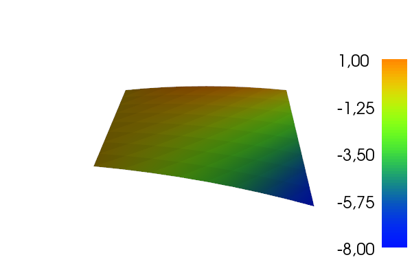 #
#
#
#
#
#
# ### Dissection of the code
#
# The function `approx` is a general solver function for any $f$ and
# $V$. We define the unknown $u$ in the variational form $a=a(u,v) = \int uv{\, \mathrm{d}x}$
# as a `TrialFunction` object and the test function $v$ as a
# `TestFunction` object. Then we define the variational form through
# the integrand `u*v*dx`. The linear form $L$ is similarly defined as
# `f*v*dx`. Here, `f` is an `Expression` object in FEniCS, i.e., a
# formula defined in terms of a C++ expression. This expression is in turn
# jit-compiled into a Python object for fast evaluation. With `a` and `L` defined,
# we re-define `u` to be a finite element function `Function`, which is
# now the unknown scalar field to be computed by the simple expression
# `solve(a == L, u)`. We remark that the above function `approx`
# is implemented in FEniCS (in a slightly more general fashion)
# in the function `project`.
#
# The `problem` function applies `approx` to solve a specific problem.
#
# ### Integrating SymPy and FEniCS
#
# The definition of $f$ must be expressed in C++. This part requires
# two definitions: one of $f$ and one of $\Omega$, or more precisely:
# the mesh (discrete $\Omega$ divided into cells). The definition of
# $f$ is here expressed in C++ (it will be compiled for fast
# evaluation), where the independent coordinates are given by a C/C++
# vector `x`. This means that $x$ is `x[0]`, $y$ is `x[1]`, and $z$ is
# `x[2]`. Moreover, `x[0]**2` must be written as `pow(x[0], 2)` in
# C/C++.
#
# Fortunately, we can easily integrate SymPy and `Expression` objects,
# because SymPy can take a formula and translate it to C/C++ code, and
# then we can require a Python code to numerically evaluate the formula.
# Here is how we can specify `f` in SymPy and use it in FEniCS as an
# `Expression` object:
# In[10]:
import sympy as sym
x, y = sym.symbols('x[0] x[1]')
f = 2*x*y - x**2
print(f)
# In[11]:
f = sym.printing.ccode(f) # Translate to C code
print(f)
# Here, the function `ccode` generates C code and we use
# `x` and `y` as placeholders for
# `x[0]` and `x[1]`, which represent the coordinate of
# a general point `x` in any dimension. The output of `ccode`
# can then be used directly in `Expression`.
#
#
# ## Refined code with curve plotting
#
#
# ### Interpolation and projection
#
# The operation of defining `a`, `L`, and solving for a `u` is so
# common that it has been implemented in the FEniCS function `project`:
# In[99]:
u = project(f, V)
# So, there is no need for our `approx` function!
#
# If we want to do interpolation (or collocation) instead, we simply do
# In[100]:
u = interpolate(f, V)
# ### Plotting the solution along a line
#
# Having `u` and `f` available as finite element functions (`Function`
# objects), we can easily plot the solution along a line since FEniCS
# has functionality for evaluating a `Function` at arbitrary points
# *inside the domain*. For example, here is the code for plotting $u$ and
# $f$ along a line $x=\hbox{const}$ or $y=\hbox{const}$.
# In[101]:
import numpy as np
import matplotlib.pyplot as plt
def comparison_plot2D(
u, f, # Function expressions in x and y
value=0.5, # x or y equals this value
variation='y', # independent variable
n=100, # no of intervals in plot
tol=1E-8, # tolerance for points inside the domain
plottitle='', # heading in plot
filename='tmp', # stem of filename
):
"""
Plot u and f along a line in x or y dir with n intervals
and a tolerance of tol for points inside the domain.
"""
v = np.linspace(-1+tol, 1-tol, n+1)
# Compute points along specified line:
points = np.array([(value, v_)
if variation == 'y' else (v_, value)
for v_ in v])
u_values = [u(point) for point in points] # eval. Function
f_values = [f(point) for point in points]
plt.figure()
plt.plot(v, u_values, 'r-', v, f_values, 'b--')
plt.legend(['u', 'f'], loc='upper left')
if variation == 'y':
plt.xlabel('y'); plt.ylabel('u, f')
else:
plt.xlabel('x'); plt.ylabel('u, f')
plt.title(plottitle)
plt.savefig(filename + '.pdf')
plt.savefig(filename + '.png')
# ### Integrating plotting and computations
#
# It is now very easy to give some graphical impression of the approximations
# for various kinds of 2D elements.
# Basically, to solve the problem of approximating $f=2xy-x^2$ on $\Omega = [-1,1]\times [0,2]$ by P2 elements on a $2\times 2$ mesh,
# we want to integrate the function above with following type of computations:
# In[102]:
import fenics as fe
f = fe.Expression('2*x[0]*x[1] - pow(x[0], 2)', degree=2)
mesh = fe.RectangleMesh(fe.Point(1,-1), fe.Point(2,1), 2, 2)
V = fe.FunctionSpace(mesh, 'P', 2)
u = fe.project(f, V)
err = fe.errornorm(f, u, 'L2')
print(err)
# However, we can now easily compare different type of elements and
# mesh resolutions:
# In[103]:
import fenics as fe
import sympy as sym
x, y = sym.symbols('x[0] x[1]')
def problem(f, nx=8, ny=8, degrees=[1,2]):
"""
Plot u along x=const or y=const for Lagrange elements,
of given degrees, on a nx times ny mesh. f is a SymPy expression.
"""
f = sym.printing.ccode(f)
f = fe.Expression(f, degree=2)
mesh = fe.RectangleMesh(
fe.Point(-1, 0), fe.Point(1, 2), 2, 2)
for degree in degrees:
if degree == 0:
# The P0 element is specified like this in FEniCS
V = fe.FunctionSpace(mesh, 'DG', 0)
else:
# The Lagrange Pd family of elements, d=1,2,3,...
V = fe.FunctionSpace(mesh, 'P', degree)
u = fe.project(f, V)
u_error = fe.errornorm(f, u, 'L2')
print(('||u-f||=%g' % u_error, degree))
comparison_plot2D(
u, f,
n=50,
value=0.4, variation='x',
plottitle='Approximation by P%d elements' % degree,
filename='approx_fenics_by_P%d' % degree,
tol=1E-3)
#fe.plot(u, title='Approx by P%d' % degree)
if __name__ == '__main__':
# x and y are global SymPy variables
f = 2*x*y - x**16
f = 2*x*y - x**2
problem(f, nx=2, ny=2, degrees=[0, 1, 2])
plt.show()
# (We note that this code issues a lot of warnings from the `u(point)`
# evaluations.)
#
# We show in [Figure](#fem:approx:fenics:2D:2:fig1)
# how $f$ is approximated by P0, P1, and P2 elements
# on a very coarse $2\times 2$ mesh consisting of 8 cells.
#
# We have also added the result obtained by P2 elements.
#
#
#
#
#
#
#
#
#
#
#
#
# ### Dissection of the code
#
# The function `approx` is a general solver function for any $f$ and
# $V$. We define the unknown $u$ in the variational form $a=a(u,v) = \int uv{\, \mathrm{d}x}$
# as a `TrialFunction` object and the test function $v$ as a
# `TestFunction` object. Then we define the variational form through
# the integrand `u*v*dx`. The linear form $L$ is similarly defined as
# `f*v*dx`. Here, `f` is an `Expression` object in FEniCS, i.e., a
# formula defined in terms of a C++ expression. This expression is in turn
# jit-compiled into a Python object for fast evaluation. With `a` and `L` defined,
# we re-define `u` to be a finite element function `Function`, which is
# now the unknown scalar field to be computed by the simple expression
# `solve(a == L, u)`. We remark that the above function `approx`
# is implemented in FEniCS (in a slightly more general fashion)
# in the function `project`.
#
# The `problem` function applies `approx` to solve a specific problem.
#
# ### Integrating SymPy and FEniCS
#
# The definition of $f$ must be expressed in C++. This part requires
# two definitions: one of $f$ and one of $\Omega$, or more precisely:
# the mesh (discrete $\Omega$ divided into cells). The definition of
# $f$ is here expressed in C++ (it will be compiled for fast
# evaluation), where the independent coordinates are given by a C/C++
# vector `x`. This means that $x$ is `x[0]`, $y$ is `x[1]`, and $z$ is
# `x[2]`. Moreover, `x[0]**2` must be written as `pow(x[0], 2)` in
# C/C++.
#
# Fortunately, we can easily integrate SymPy and `Expression` objects,
# because SymPy can take a formula and translate it to C/C++ code, and
# then we can require a Python code to numerically evaluate the formula.
# Here is how we can specify `f` in SymPy and use it in FEniCS as an
# `Expression` object:
# In[10]:
import sympy as sym
x, y = sym.symbols('x[0] x[1]')
f = 2*x*y - x**2
print(f)
# In[11]:
f = sym.printing.ccode(f) # Translate to C code
print(f)
# Here, the function `ccode` generates C code and we use
# `x` and `y` as placeholders for
# `x[0]` and `x[1]`, which represent the coordinate of
# a general point `x` in any dimension. The output of `ccode`
# can then be used directly in `Expression`.
#
#
# ## Refined code with curve plotting
#
#
# ### Interpolation and projection
#
# The operation of defining `a`, `L`, and solving for a `u` is so
# common that it has been implemented in the FEniCS function `project`:
# In[99]:
u = project(f, V)
# So, there is no need for our `approx` function!
#
# If we want to do interpolation (or collocation) instead, we simply do
# In[100]:
u = interpolate(f, V)
# ### Plotting the solution along a line
#
# Having `u` and `f` available as finite element functions (`Function`
# objects), we can easily plot the solution along a line since FEniCS
# has functionality for evaluating a `Function` at arbitrary points
# *inside the domain*. For example, here is the code for plotting $u$ and
# $f$ along a line $x=\hbox{const}$ or $y=\hbox{const}$.
# In[101]:
import numpy as np
import matplotlib.pyplot as plt
def comparison_plot2D(
u, f, # Function expressions in x and y
value=0.5, # x or y equals this value
variation='y', # independent variable
n=100, # no of intervals in plot
tol=1E-8, # tolerance for points inside the domain
plottitle='', # heading in plot
filename='tmp', # stem of filename
):
"""
Plot u and f along a line in x or y dir with n intervals
and a tolerance of tol for points inside the domain.
"""
v = np.linspace(-1+tol, 1-tol, n+1)
# Compute points along specified line:
points = np.array([(value, v_)
if variation == 'y' else (v_, value)
for v_ in v])
u_values = [u(point) for point in points] # eval. Function
f_values = [f(point) for point in points]
plt.figure()
plt.plot(v, u_values, 'r-', v, f_values, 'b--')
plt.legend(['u', 'f'], loc='upper left')
if variation == 'y':
plt.xlabel('y'); plt.ylabel('u, f')
else:
plt.xlabel('x'); plt.ylabel('u, f')
plt.title(plottitle)
plt.savefig(filename + '.pdf')
plt.savefig(filename + '.png')
# ### Integrating plotting and computations
#
# It is now very easy to give some graphical impression of the approximations
# for various kinds of 2D elements.
# Basically, to solve the problem of approximating $f=2xy-x^2$ on $\Omega = [-1,1]\times [0,2]$ by P2 elements on a $2\times 2$ mesh,
# we want to integrate the function above with following type of computations:
# In[102]:
import fenics as fe
f = fe.Expression('2*x[0]*x[1] - pow(x[0], 2)', degree=2)
mesh = fe.RectangleMesh(fe.Point(1,-1), fe.Point(2,1), 2, 2)
V = fe.FunctionSpace(mesh, 'P', 2)
u = fe.project(f, V)
err = fe.errornorm(f, u, 'L2')
print(err)
# However, we can now easily compare different type of elements and
# mesh resolutions:
# In[103]:
import fenics as fe
import sympy as sym
x, y = sym.symbols('x[0] x[1]')
def problem(f, nx=8, ny=8, degrees=[1,2]):
"""
Plot u along x=const or y=const for Lagrange elements,
of given degrees, on a nx times ny mesh. f is a SymPy expression.
"""
f = sym.printing.ccode(f)
f = fe.Expression(f, degree=2)
mesh = fe.RectangleMesh(
fe.Point(-1, 0), fe.Point(1, 2), 2, 2)
for degree in degrees:
if degree == 0:
# The P0 element is specified like this in FEniCS
V = fe.FunctionSpace(mesh, 'DG', 0)
else:
# The Lagrange Pd family of elements, d=1,2,3,...
V = fe.FunctionSpace(mesh, 'P', degree)
u = fe.project(f, V)
u_error = fe.errornorm(f, u, 'L2')
print(('||u-f||=%g' % u_error, degree))
comparison_plot2D(
u, f,
n=50,
value=0.4, variation='x',
plottitle='Approximation by P%d elements' % degree,
filename='approx_fenics_by_P%d' % degree,
tol=1E-3)
#fe.plot(u, title='Approx by P%d' % degree)
if __name__ == '__main__':
# x and y are global SymPy variables
f = 2*x*y - x**16
f = 2*x*y - x**2
problem(f, nx=2, ny=2, degrees=[0, 1, 2])
plt.show()
# (We note that this code issues a lot of warnings from the `u(point)`
# evaluations.)
#
# We show in [Figure](#fem:approx:fenics:2D:2:fig1)
# how $f$ is approximated by P0, P1, and P2 elements
# on a very coarse $2\times 2$ mesh consisting of 8 cells.
#
# We have also added the result obtained by P2 elements.
#
#
#
#
#
# Comparison of P0, P1, and P2 approximations (left to right) along a line in a 2D mesh.
#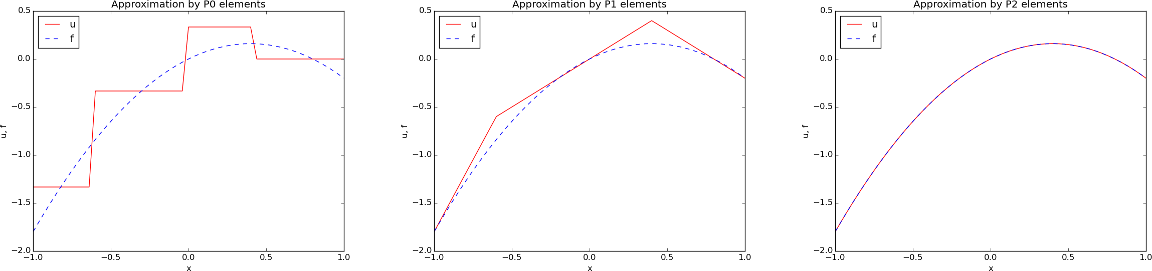 #
#
#
#