#!/usr/bin/env python
# coding: utf-8

# <center><div style="direction:rtl;font-family:B Lotus, B Nazanin, Tahoma">به نام خدا</div></center>
# <h1><center><div style="direction:rtl;font-family:B Lotus, B Nazanin, Tahoma">آموزش یک شبکه عصبی کانولوشنالی از ابتدا</div></center></h1>

# In[1]:


import keras


# # <div style="direction:rtl;text-align:right;font-family:B Lotus, B Nazanin, Tahoma">آموزش یک شبکه عصبی کانولوشنالی از ابتدا</div>
# 
# <div style="direction:rtl;text-align:right;font-family:Tahoma">
# کدها  برگرفته از فصل دو کتاب
# </div>
# 
# [Deep Learning with Python](https://www.manning.com/books/deep-learning-with-python?a_aid=keras&a_bid=76564dff)
# <div style="direction:rtl;text-align:right;font-family:Tahoma">
# و گیت هاب نویسنده کتاب و توسعه دهنده کراس 
# </div>
# 
# [François Chollet](http://nbviewer.jupyter.org/github/fchollet/deep-learning-with-python-notebooks/blob/master/5.2-using-convnets-with-small-datasets.ipynb)
# <div style="direction:rtl;text-align:right;font-family:Tahoma">
# است.
# </div>
# 

# # <div style="direction:rtl;text-align:right;font-family:B Lotus, B Nazanin, Tahoma">مجموعه داده</div>
# 
# <div style="direction:rtl;text-align:right;font-family:Tahoma">
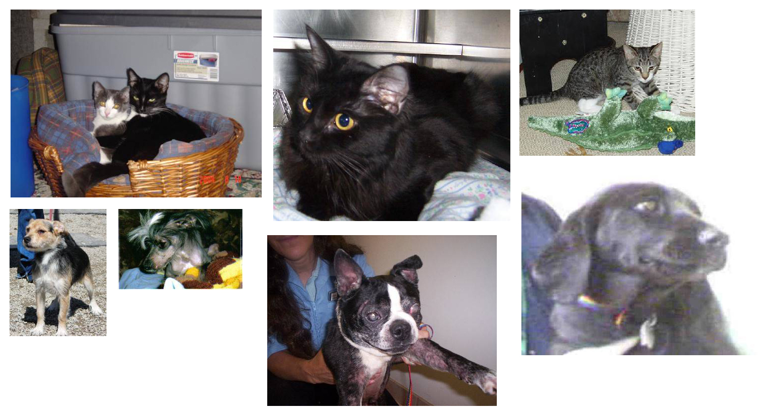
# مجموعه داده گربه در مقابل سگ برای این مثال استفاده شده است. این مجموعه داده در چالش بینایی کامپیوتر اواخر سال ۲۰۱۳ توسط سایت Kaggle.com در دسترس عموم قرار گرفت.
# <br>
# از قبل از سال ۲۰۱۳ استفاده از شبکه های کانولوشنالی خیلی رایج نبود.
# مجموعه داده در آدرس زیر قابل دانلود است.
# </div>
# 
# `https://www.kaggle.com/c/dogs-vs-cats/data`
# 
# 
# 
# ![cats_vs_dogs_samples](https://s3.amazonaws.com/book.keras.io/img/ch5/cats_vs_dogs_samples.jpg)

# Unsurprisingly, the cats vs. dogs Kaggle competition in 2013 was won by entrants who used convnets. The best entries could achieve up to 
# 95% accuracy. In our own example, we will get fairly close to this accuracy (in the next section), even though we will be training our 
# models on less than 10% of the data that was available to the competitors.
# This original dataset contains 25,000 images of dogs and cats (12,500 from each class) and is 543MB large (compressed). After downloading 
# and uncompressing it, we will create a new dataset containing three subsets: a training set with 1000 samples of each class, a validation 
# set with 500 samples of each class, and finally a test set with 500 samples of each class.
# 
# Here are a few lines of code to do this:

# In[2]:


import os, shutil


# In[3]:


# The path to the directory where the original
# dataset was uncompressed
original_dataset_dir = 'D:/dataset/catDog/train'

# The directory where we will
# store our smaller dataset
base_dir = 'D:/dataset/catDog/catVsdog'
os.mkdir(base_dir)

# Directories for our training,
# validation and test splits
train_dir = os.path.join(base_dir, 'train')
os.mkdir(train_dir)
validation_dir = os.path.join(base_dir, 'validation')
os.mkdir(validation_dir)
test_dir = os.path.join(base_dir, 'test')
os.mkdir(test_dir)

# Directory with our training cat pictures
train_cats_dir = os.path.join(train_dir, 'cats')
os.mkdir(train_cats_dir)

# Directory with our training dog pictures
train_dogs_dir = os.path.join(train_dir, 'dogs')
os.mkdir(train_dogs_dir)

# Directory with our validation cat pictures
validation_cats_dir = os.path.join(validation_dir, 'cats')
os.mkdir(validation_cats_dir)

# Directory with our validation dog pictures
validation_dogs_dir = os.path.join(validation_dir, 'dogs')
os.mkdir(validation_dogs_dir)

# Directory with our validation cat pictures
test_cats_dir = os.path.join(test_dir, 'cats')
os.mkdir(test_cats_dir)

# Directory with our validation dog pictures
test_dogs_dir = os.path.join(test_dir, 'dogs')
os.mkdir(test_dogs_dir)

# Copy first 1000 cat images to train_cats_dir
fnames = ['cat.{}.jpg'.format(i) for i in range(1000)]
for fname in fnames:
    src = os.path.join(original_dataset_dir, fname)
    dst = os.path.join(train_cats_dir, fname)
    shutil.copyfile(src, dst)

# Copy next 500 cat images to validation_cats_dir
fnames = ['cat.{}.jpg'.format(i) for i in range(1000, 1500)]
for fname in fnames:
    src = os.path.join(original_dataset_dir, fname)
    dst = os.path.join(validation_cats_dir, fname)
    shutil.copyfile(src, dst)
    
# Copy next 500 cat images to test_cats_dir
fnames = ['cat.{}.jpg'.format(i) for i in range(1500, 2000)]
for fname in fnames:
    src = os.path.join(original_dataset_dir, fname)
    dst = os.path.join(test_cats_dir, fname)
    shutil.copyfile(src, dst)
    
# Copy first 1000 dog images to train_dogs_dir
fnames = ['dog.{}.jpg'.format(i) for i in range(1000)]
for fname in fnames:
    src = os.path.join(original_dataset_dir, fname)
    dst = os.path.join(train_dogs_dir, fname)
    shutil.copyfile(src, dst)
    
# Copy next 500 dog images to validation_dogs_dir
fnames = ['dog.{}.jpg'.format(i) for i in range(1000, 1500)]
for fname in fnames:
    src = os.path.join(original_dataset_dir, fname)
    dst = os.path.join(validation_dogs_dir, fname)
    shutil.copyfile(src, dst)
    
# Copy next 500 dog images to test_dogs_dir
fnames = ['dog.{}.jpg'.format(i) for i in range(1500, 2000)]
for fname in fnames:
    src = os.path.join(original_dataset_dir, fname)
    dst = os.path.join(test_dogs_dir, fname)
    shutil.copyfile(src, dst)


# ## <div style="direction:rtl;text-align:right;font-family:B Lotus, B Nazanin, Tahoma"> برای بررسی صحت انجام کار تعداد تصاویرآموزشی/آزمون/توسعه را بررسی میکنیم.</div>
# 

# In[4]:


train_cats_dir


# In[5]:


print('total training cat images:', len(os.listdir(train_cats_dir)))


# In[6]:


print('total training dog images:', len(os.listdir(train_dogs_dir)))


# In[7]:


print('total validation cat images:', len(os.listdir(validation_cats_dir)))


# In[8]:


print('total validation dog images:', len(os.listdir(validation_dogs_dir)))


# In[9]:


print('total test cat images:', len(os.listdir(test_cats_dir)))


# In[10]:


print('total test dog images:', len(os.listdir(test_dogs_dir)))


# <div style="direction:rtl;text-align:right;font-family:Tahoma">
# با توجه به اینکه تعداد تصاویر یکسانی از سگ و گربه برداشته ایم معیار Accuracy معیارمناسبی برای ارزیابی خواهد بود.
# </div>

# ## <div style="direction:rtl;text-align:right;font-family:B Lotus, B Nazanin, Tahoma">تعریف معماری مدل (model architecture)</div>
# 
# Since we are attacking a binary classification problem, we are ending the network with a single unit (a `Dense` layer of size 1) and a 
# `sigmoid` activation. This unit will encode the probability that the network is looking at one class or the other.

# In[13]:


from keras import layers
from keras import models

model = models.Sequential()
model.add(layers.Conv2D(32, (3, 3), activation='relu',
                        input_shape=(150, 150, 3)))
model.add(layers.MaxPooling2D((2, 2)))
model.add(layers.Conv2D(64, (3, 3), activation='relu'))
model.add(layers.MaxPooling2D((2, 2)))
model.add(layers.Conv2D(128, (3, 3), activation='relu'))
model.add(layers.MaxPooling2D((2, 2)))
model.add(layers.Conv2D(128, (3, 3), activation='relu'))
model.add(layers.MaxPooling2D((2, 2)))
model.add(layers.Flatten())
model.add(layers.Dense(512, activation='relu'))
model.add(layers.Dense(1, activation='sigmoid'))


# Let's take a look at how the dimensions of the feature maps change with every successive layer:

# In[14]:


model.summary()


# For our compilation step, we'll go with the `RMSprop` optimizer as usual. Since we ended our network with a single sigmoid unit, we will 
# use binary crossentropy as our loss (as a reminder, check out the table in Chapter 4, section 5 for a cheatsheet on what loss function to 
# use in various situations).

# In[15]:


from keras import optimizers

model.compile(loss='binary_crossentropy',
              optimizer=optimizers.RMSprop(lr=1e-4),
              metrics=['acc'])


# ## <div style="direction:rtl;text-align:right;font-family:B Lotus, B Nazanin, Tahoma">  پیش پردازش داده (Data preprocessing)</div>
# 
# * Read the picture files.
# * Decode the JPEG content to RGB grids of pixels.
# * Convert these into floating point tensors.
# * Rescale the pixel values (between 0 and 255) to the [0, 1] interval (as you know, neural networks prefer to deal with small input values).
# 
# It may seem a bit daunting, but thankfully Keras has utilities to take care of these steps automatically. Keras has a module with image 
# processing helper tools, located at `keras.preprocessing.image`. In particular, it contains the class `ImageDataGenerator` which allows to 
# quickly set up Python generators that can automatically turn image files on disk into batches of pre-processed tensors. This is what we 
# will use here.
# 
# <div style="direction:rtl;text-align:right;font-family:Tahoma">
#     اطلاعات بیشتر در مستندات Keras :
# </div>
# 
# `https://keras.io/preprocessing/image/`

# In[16]:


from keras.preprocessing.image import ImageDataGenerator

# All images will be rescaled by 1./255
train_datagen = ImageDataGenerator(rescale=1./255)
test_datagen = ImageDataGenerator(rescale=1./255)

train_generator = train_datagen.flow_from_directory(
        # This is the target directory
        train_dir,
        # All images will be resized to 150x150
        target_size=(150, 150),
        batch_size=20,
        # Since we use binary_crossentropy loss, we need binary labels
        class_mode='binary')

validation_generator = test_datagen.flow_from_directory(
        validation_dir,
        target_size=(150, 150),
        batch_size=20,
        class_mode='binary')


# Let's take a look at the output of one of these generators: it yields batches of 150x150 RGB images (shape `(20, 150, 150, 3)`) and binary 
# labels (shape `(20,)`). 20 is the number of samples in each batch (the batch size). Note that the generator yields these batches 
# indefinitely: it just loops endlessly over the images present in the target folder. For this reason, we need to `break` the iteration loop 
# at some point.

# In[17]:


for data_batch, labels_batch in train_generator:
    print('data batch shape:', data_batch.shape)
    print('labels batch shape:', labels_batch.shape)
    break


# Let's fit our model to the data using the generator. We do it using the `fit_generator` method, the equivalent of `fit` for data generators 
# like ours. It expects as first argument a Python generator that will yield batches of inputs and targets indefinitely, like ours does. 
# Because the data is being generated endlessly, the generator needs to know example how many samples to draw from the generator before 
# declaring an epoch over. This is the role of the `steps_per_epoch` argument: after having drawn `steps_per_epoch` batches from the 
# generator, i.e. after having run for `steps_per_epoch` gradient descent steps, the fitting process will go to the next epoch. In our case, 
# batches are 20-sample large, so it will take 100 batches until we see our target of 2000 samples.
# 
# When using `fit_generator`, one may pass a `validation_data` argument, much like with the `fit` method. Importantly, this argument is 
# allowed to be a data generator itself, but it could be a tuple of Numpy arrays as well. If you pass a generator as `validation_data`, then 
# this generator is expected to yield batches of validation data endlessly, and thus you should also specify the `validation_steps` argument, 
# which tells the process how many batches to draw from the validation generator for evaluation.

# In[15]:


history = model.fit_generator(
      train_generator,
      steps_per_epoch=100,
      epochs=30,
      validation_data=validation_generator,
      validation_steps=50)


# Let's plot the loss and accuracy of the model over the training and validation data during training:

# In[16]:


import matplotlib.pyplot as plt
get_ipython().run_line_magic('matplotlib', 'inline')
acc = history.history['acc']
val_acc = history.history['val_acc']
loss = history.history['loss']
val_loss = history.history['val_loss']

epochs = range(len(acc))

plt.plot(epochs, acc, 'bo', label='Training acc')
plt.plot(epochs, val_acc, 'b', label='Validation acc')
plt.title('Training and validation accuracy')
plt.legend()

plt.figure()

plt.plot(epochs, loss, 'bo', label='Training loss')
plt.plot(epochs, val_loss, 'b', label='Validation loss')
plt.title('Training and validation loss')
plt.legend()

plt.show()


# These plots are characteristic of overfitting. Our training accuracy increases linearly over time, until it reaches nearly 100%, while our 
# validation accuracy stalls at 70-72%. Our validation loss reaches its minimum after only five epochs then stalls, while the training loss 
# keeps decreasing linearly until it reaches nearly 0.
# 
# Because we only have relatively few training samples (2000), overfitting is going to be our number one concern.
# Let's train our network using data augmentation and dropout:

# ## <div style="direction:rtl;text-align:right;font-family:B Lotus, B Nazanin, Tahoma">شبکه با Dropout</div>

# In[17]:


model = models.Sequential()
model.add(layers.Conv2D(32, (3, 3), activation='relu',
                        input_shape=(150, 150, 3)))
model.add(layers.MaxPooling2D((2, 2)))
model.add(layers.Conv2D(64, (3, 3), activation='relu'))
model.add(layers.MaxPooling2D((2, 2)))
model.add(layers.Conv2D(128, (3, 3), activation='relu'))
model.add(layers.MaxPooling2D((2, 2)))
model.add(layers.Conv2D(128, (3, 3), activation='relu'))
model.add(layers.MaxPooling2D((2, 2)))
model.add(layers.Flatten())
model.add(layers.Dropout(0.5))
model.add(layers.Dense(512, activation='relu'))
model.add(layers.Dense(1, activation='sigmoid'))

model.compile(loss='binary_crossentropy',
              optimizer=optimizers.RMSprop(lr=1e-4),
              metrics=['acc'])

history = model.fit_generator(
      train_generator,
      steps_per_epoch=100,
      epochs=100,
      validation_data=validation_generator,
      validation_steps=50)


# Let's plot our results again:

# In[18]:


acc = history.history['acc']
val_acc = history.history['val_acc']
loss = history.history['loss']
val_loss = history.history['val_loss']

epochs = range(len(acc))

plt.plot(epochs, acc, 'bo', label='Training acc')
plt.plot(epochs, val_acc, 'b', label='Validation acc')
plt.title('Training and validation accuracy')
plt.legend()

plt.figure()

plt.plot(epochs, loss, 'bo', label='Training loss')
plt.plot(epochs, val_loss, 'b', label='Validation loss')
plt.title('Training and validation loss')
plt.legend()

plt.show()


# ## <div style="direction:rtl;text-align:right;font-family:B Lotus, B Nazanin, Tahoma">ذخیره کردن مدل</div>
# 

# In[19]:


model.save('cats_and_dogs_small_1.h5')


# <div class="alert alert-block alert-info">
# <div style="direction:rtl;text-align:right;font-family:B Lotus, B Nazanin, Tahoma"> دوره مقدماتی یادگیری عمیق<br>علیرضا اخوان پور<br>پنج شنبه، ۲۵ بهمن ۱۳۹۷<br>
# </div>
# <a href="http://class.vision">Class.Vision</a> - <a href="http://AkhavanPour.ir">AkhavanPour.ir</a> - <a href="https://github.com/Alireza-Akhavan/">GitHub</a>
# 
# </div>

# In[ ]: