#!/usr/bin/env python
# coding: utf-8
# # Advanced MLP
# - Advanced techniques for training neural networks
# - Weight Initialization
# - Nonlinearity (Activation function)
# - Optimizers
# - Batch Normalization
# - Dropout (Regularization)
# - Model Ensemble
# In[ ]:
import matplotlib.pyplot as plt
from sklearn.model_selection import train_test_split
from tensorflow.keras.datasets import mnist
from tensorflow.keras.models import Sequential
from tensorflow.keras.utils import to_categorical
# ## Load Dataset
# - MNIST dataset
# - source: http://yann.lecun.com/exdb/mnist/
# In[ ]:
(X_train, y_train), (X_test, y_test) = mnist.load_data()
# In[ ]:
plt.imshow(X_train[0]) # show first number in the dataset
plt.show()
print('Label: ', y_train[0])
# In[ ]:
plt.imshow(X_test[0]) # show first number in the dataset
plt.show()
print('Label: ', y_test[0])
# In[ ]:
# reshaping X data: (n, 28, 28) => (n, 784)
X_train = X_train.reshape((X_train.shape[0], -1))
X_test = X_test.reshape((X_test.shape[0], -1))
# In[ ]:
# converting y data into categorical (one-hot encoding)
y_train = to_categorical(y_train)
y_test = to_categorical(y_test)
# In[ ]:
print(X_train.shape, X_test.shape, y_train.shape, y_test.shape)
# ## Basic MLP model
# - Naive MLP model without any alterations
# In[ ]:
from tensorflow.keras.models import Sequential
from tensorflow.keras.layers import Activation, Dense
from tensorflow.keras import optimizers
# In[ ]:
model = Sequential()
# In[ ]:
model.add(Dense(50, input_shape = (784, )))
model.add(Activation('sigmoid'))
model.add(Dense(50))
model.add(Activation('sigmoid'))
model.add(Dense(50))
model.add(Activation('sigmoid'))
model.add(Dense(50))
model.add(Activation('sigmoid'))
model.add(Dense(10))
model.add(Activation('softmax'))
# In[ ]:
sgd = optimizers.SGD(lr = 0.001)
model.compile(optimizer = sgd, loss = 'categorical_crossentropy', metrics = ['accuracy'])
# In[ ]:
history = model.fit(X_train, y_train, batch_size = 256, validation_split = 0.3, epochs = 100, verbose = 1)
# In[ ]:
plt.plot(history.history['accuracy'])
plt.plot(history.history['val_accuracy'])
plt.plot(history.history['loss'])
plt.plot(history.history['val_loss'])
plt.legend(['train acc', 'valid acc', 'train loss', 'valid loss'], loc = 'upper left')
plt.show()
# Training and validation accuracy seems to improve after around 60 epochs
# In[ ]:
results = model.evaluate(X_test, y_test)
# In[ ]:
print('Test accuracy: ', results[1])
# ## 1. Weight Initialization
# - Changing weight initialization scheme can sometimes improve training of the model by preventing vanishing gradient problem up to some degree
# - He normal or Xavier normal initialization schemes are SOTA at the moment
# - Doc: https://keras.io/initializers/
# In[ ]:
# from now on, create a function to generate (return) models
def mlp_model():
model = Sequential()
model.add(Dense(50, input_shape = (784, ), kernel_initializer='he_normal')) # use he_normal initializer
model.add(Activation('sigmoid'))
model.add(Dense(50, kernel_initializer='he_normal')) # use he_normal initializer
model.add(Activation('sigmoid'))
model.add(Dense(50, kernel_initializer='he_normal')) # use he_normal initializer
model.add(Activation('sigmoid'))
model.add(Dense(50, kernel_initializer='he_normal')) # use he_normal initializer
model.add(Activation('sigmoid'))
model.add(Dense(10, kernel_initializer='he_normal')) # use he_normal initializer
model.add(Activation('softmax'))
sgd = optimizers.SGD(lr = 0.001)
model.compile(optimizer = sgd, loss = 'categorical_crossentropy', metrics = ['accuracy'])
return model
# In[ ]:
model = mlp_model()
history = model.fit(X_train, y_train, validation_split = 0.3, epochs = 100, verbose = 1)
# In[ ]:
plt.plot(history.history['accuracy'])
plt.plot(history.history['val_accuracy'])
plt.plot(history.history['loss'])
plt.plot(history.history['val_loss'])
plt.legend(['train acc', 'valid acc', 'train loss', 'valid loss'], loc = 'upper left')
plt.show()
# Training and validation accuracy seems to improve after around 60 epochs
# In[ ]:
results = model.evaluate(X_test, y_test)
# In[ ]:
print('Test accuracy: ', results[1])
# ## 2. Nonlinearity (Activation function)
# - Sigmoid functions suffer from gradient vanishing problem, making training slower
# - There are many choices apart from sigmoid and tanh; try many of them!
# - **'relu'** (rectified linear unit) is one of the most popular ones
# - **'selu'** (scaled exponential linear unit) is one of the most recent ones
# - Doc: https://keras.io/activations/
# 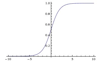 # **Sigmoid Activation Function**
#
# **Sigmoid Activation Function**
# 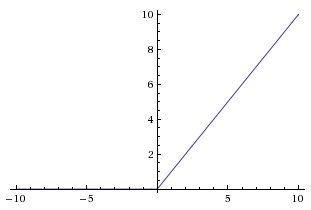 # **Relu Activation Function**
# In[ ]:
def mlp_model():
model = Sequential()
model.add(Dense(50, input_shape = (784, )))
model.add(Activation('relu')) # use relu
model.add(Dense(50))
model.add(Activation('relu')) # use relu
model.add(Dense(50))
model.add(Activation('relu')) # use relu
model.add(Dense(50))
model.add(Activation('relu')) # use relu
model.add(Dense(10))
model.add(Activation('softmax'))
sgd = optimizers.SGD(lr = 0.001)
model.compile(optimizer = sgd, loss = 'categorical_crossentropy', metrics = ['accuracy'])
return model
# In[ ]:
model = mlp_model()
history = model.fit(X_train, y_train, validation_split = 0.3, epochs = 100, verbose = 1)
# In[ ]:
plt.plot(history.history['accuracy'])
plt.plot(history.history['val_accuracy'])
plt.plot(history.history['loss'])
plt.plot(history.history['val_loss'])
plt.legend(['train acc', 'valid acc', 'train loss', 'valid loss'], loc = 'upper left')
plt.show()
# Training and validation accuracy improve instantaneously, but reach a plateau after around 30 epochs
# In[ ]:
results = model.evaluate(X_test, y_test)
# In[ ]:
print('Test accuracy: ', results[1])
# ## 3. Optimizers
# - Many variants of SGD are proposed and employed nowadays
# - One of the most popular ones are Adam (Adaptive Moment Estimation)
# - Doc: https://keras.io/optimizers/
#
# **Relu Activation Function**
# In[ ]:
def mlp_model():
model = Sequential()
model.add(Dense(50, input_shape = (784, )))
model.add(Activation('relu')) # use relu
model.add(Dense(50))
model.add(Activation('relu')) # use relu
model.add(Dense(50))
model.add(Activation('relu')) # use relu
model.add(Dense(50))
model.add(Activation('relu')) # use relu
model.add(Dense(10))
model.add(Activation('softmax'))
sgd = optimizers.SGD(lr = 0.001)
model.compile(optimizer = sgd, loss = 'categorical_crossentropy', metrics = ['accuracy'])
return model
# In[ ]:
model = mlp_model()
history = model.fit(X_train, y_train, validation_split = 0.3, epochs = 100, verbose = 1)
# In[ ]:
plt.plot(history.history['accuracy'])
plt.plot(history.history['val_accuracy'])
plt.plot(history.history['loss'])
plt.plot(history.history['val_loss'])
plt.legend(['train acc', 'valid acc', 'train loss', 'valid loss'], loc = 'upper left')
plt.show()
# Training and validation accuracy improve instantaneously, but reach a plateau after around 30 epochs
# In[ ]:
results = model.evaluate(X_test, y_test)
# In[ ]:
print('Test accuracy: ', results[1])
# ## 3. Optimizers
# - Many variants of SGD are proposed and employed nowadays
# - One of the most popular ones are Adam (Adaptive Moment Estimation)
# - Doc: https://keras.io/optimizers/
#  #
#
**Relative convergence speed of different optimizers**
# In[ ]:
def mlp_model():
model = Sequential()
model.add(Dense(50, input_shape = (784, )))
model.add(Activation('sigmoid'))
model.add(Dense(50))
model.add(Activation('sigmoid'))
model.add(Dense(50))
model.add(Activation('sigmoid'))
model.add(Dense(50))
model.add(Activation('sigmoid'))
model.add(Dense(10))
model.add(Activation('softmax'))
adam = optimizers.Adam(lr = 0.001) # use Adam optimizer
model.compile(optimizer = adam, loss = 'categorical_crossentropy', metrics = ['accuracy'])
return model
# In[ ]:
model = mlp_model()
history = model.fit(X_train, y_train, validation_split = 0.3, epochs = 100, verbose = 0)
# In[ ]:
plt.plot(history.history['accuracy'])
plt.plot(history.history['val_accuracy'])
plt.plot(history.history['loss'])
plt.plot(history.history['val_loss'])
plt.legend(['train acc', 'valid acc', 'train loss', 'valid loss'], loc = 'upper left')
plt.show()
# Training and validation accuracy improve instantaneously, but reach plateau after around 50 epochs
# In[ ]:
results = model.evaluate(X_test, y_test)
# In[ ]:
print('Test accuracy: ', results[1])
# ## 4. Batch Normalization
# - Batch Normalization, one of the methods to prevent the "internal covariance shift" problem, has proven to be highly effective
# - Normalize each mini-batch before nonlinearity
# - Doc: https://keras.io/optimizers/
# 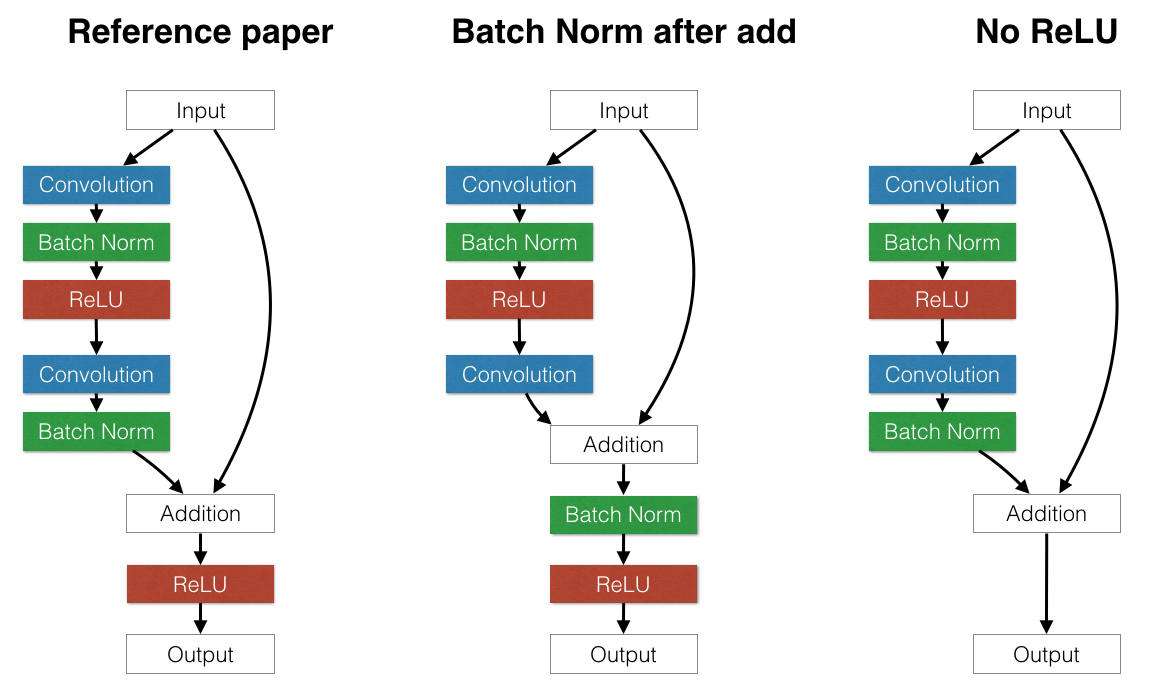 #
#
#
#
Batch normalization layer is usually inserted after dense/convolution and before nonlinearity
# In[ ]:
from keras.layers import BatchNormalization
# In[ ]:
def mlp_model():
model = Sequential()
model.add(Dense(50, input_shape = (784, )))
model.add(BatchNormalization()) # Add Batchnorm layer before Activation
model.add(Activation('sigmoid'))
model.add(Dense(50))
model.add(BatchNormalization()) # Add Batchnorm layer before Activation
model.add(Activation('sigmoid'))
model.add(Dense(50))
model.add(BatchNormalization()) # Add Batchnorm layer before Activation
model.add(Activation('sigmoid'))
model.add(Dense(50))
model.add(BatchNormalization()) # Add Batchnorm layer before Activation
model.add(Activation('sigmoid'))
model.add(Dense(10))
model.add(Activation('softmax'))
sgd = optimizers.SGD(lr = 0.001)
model.compile(optimizer = sgd, loss = 'categorical_crossentropy', metrics = ['accuracy'])
return model
# In[ ]:
model = mlp_model()
history = model.fit(X_train, y_train, validation_split = 0.3, epochs = 100, verbose = 0)
# In[ ]:
plt.plot(history.history['accuracy'])
plt.plot(history.history['val_accuracy'])
plt.plot(history.history['loss'])
plt.plot(history.history['val_loss'])
plt.legend(['train acc', 'valid acc', 'train loss', 'valid loss'], loc = 'upper left')
plt.show()
# Training and validation accuracy improve consistently, but reach plateau after around 60 epochs
# In[ ]:
results = model.evaluate(X_test, y_test)
# In[ ]:
print('Test accuracy: ', results[1])
# ## 5. Dropout (Regularization)
# - Dropout is one of powerful ways to prevent overfitting
# - The idea is simple. It is disconnecting some (randomly selected) neurons in each layer
# - The probability of each neuron to be disconnected, namely 'Dropout rate', has to be designated
# - Doc: https://keras.io/layers/core/#dropout
#  # In[ ]:
from keras.layers import Dropout
# In[ ]:
def mlp_model():
model = Sequential()
model.add(Dense(50, input_shape = (784, )))
model.add(Activation('sigmoid'))
model.add(Dropout(0.2)) # Dropout layer after Activation
model.add(Dense(50))
model.add(Activation('sigmoid'))
model.add(Dropout(0.2)) # Dropout layer after Activation
model.add(Dense(50))
model.add(Activation('sigmoid'))
model.add(Dropout(0.2)) # Dropout layer after Activation
model.add(Dense(50))
model.add(Activation('sigmoid'))
model.add(Dropout(0.2)) # Dropout layer after Activation
model.add(Dense(10))
model.add(Activation('softmax'))
sgd = optimizers.SGD(lr = 0.001)
model.compile(optimizer = sgd, loss = 'categorical_crossentropy', metrics = ['accuracy'])
return model
# In[ ]:
model = mlp_model()
history = model.fit(X_train, y_train, validation_split = 0.3, epochs = 100, verbose = 0)
# In[ ]:
plt.plot(history.history['accuracy'])
plt.plot(history.history['val_accuracy'])
plt.plot(history.history['loss'])
plt.plot(history.history['val_loss'])
plt.legend(['train acc', 'valid acc', 'train loss', 'valid loss'], loc = 'upper left')
plt.show()
# Validation results does not improve since it did not show signs of overfitting, yet.
#
# In[ ]:
from keras.layers import Dropout
# In[ ]:
def mlp_model():
model = Sequential()
model.add(Dense(50, input_shape = (784, )))
model.add(Activation('sigmoid'))
model.add(Dropout(0.2)) # Dropout layer after Activation
model.add(Dense(50))
model.add(Activation('sigmoid'))
model.add(Dropout(0.2)) # Dropout layer after Activation
model.add(Dense(50))
model.add(Activation('sigmoid'))
model.add(Dropout(0.2)) # Dropout layer after Activation
model.add(Dense(50))
model.add(Activation('sigmoid'))
model.add(Dropout(0.2)) # Dropout layer after Activation
model.add(Dense(10))
model.add(Activation('softmax'))
sgd = optimizers.SGD(lr = 0.001)
model.compile(optimizer = sgd, loss = 'categorical_crossentropy', metrics = ['accuracy'])
return model
# In[ ]:
model = mlp_model()
history = model.fit(X_train, y_train, validation_split = 0.3, epochs = 100, verbose = 0)
# In[ ]:
plt.plot(history.history['accuracy'])
plt.plot(history.history['val_accuracy'])
plt.plot(history.history['loss'])
plt.plot(history.history['val_loss'])
plt.legend(['train acc', 'valid acc', 'train loss', 'valid loss'], loc = 'upper left')
plt.show()
# Validation results does not improve since it did not show signs of overfitting, yet.
#
Hence, the key takeaway message is that apply dropout when you see a signal of overfitting.
# In[ ]:
results = model.evaluate(X_test, y_test)
# In[ ]:
print('Test accuracy: ', results[1])
# ## 6. Model Ensemble
# - Model ensemble is a reliable and promising way to boost performance of the model
# - Usually create 8 to 10 independent networks and merge their results
# - Here, we resort to scikit-learn API, **VotingClassifier**
# - Doc: http://scikit-learn.org/stable/modules/generated/sklearn.ensemble.VotingClassifier.html
#  # In[ ]:
import numpy as np
from tensorflow.keras.wrappers.scikit_learn import KerasClassifier
from sklearn.ensemble import VotingClassifier
from sklearn.metrics import accuracy_score
# In[ ]:
y_train = np.argmax(y_train, axis = 1)
y_test = np.argmax(y_test, axis = 1)
# In[ ]:
def mlp_model():
model = Sequential()
model.add(Dense(50, input_shape = (784, )))
model.add(Activation('sigmoid'))
model.add(Dense(50))
model.add(Activation('sigmoid'))
model.add(Dense(50))
model.add(Activation('sigmoid'))
model.add(Dense(50))
model.add(Activation('sigmoid'))
model.add(Dense(10))
model.add(Activation('softmax'))
sgd = optimizers.SGD(lr = 0.001)
model.compile(optimizer = sgd, loss = 'categorical_crossentropy', metrics = ['accuracy'])
return model
# In[ ]:
model1 = KerasClassifier(build_fn = mlp_model, epochs = 100, verbose = 0)
model2 = KerasClassifier(build_fn = mlp_model, epochs = 100, verbose = 0)
model3 = KerasClassifier(build_fn = mlp_model, epochs = 100, verbose = 0)
model1._estimator_type = "classifier"
model2._estimator_type = "classifier"
model3._estimator_type = "classifier"
# In[ ]:
ensemble_clf = VotingClassifier(estimators = [('model1', model1), ('model2', model2), ('model3', model3)]
, voting = 'soft')
# In[ ]:
ensemble_clf.fit(X_train, y_train)
# In[ ]:
y_pred = ensemble_clf.predict(X_test)
# In[ ]:
print('Test accuracy:', accuracy_score(y_pred, y_test))
# ## Summary
#
# Below table is a summary of evaluation results so far. It turns out that all methods improve the test performance over the MNIST dataset. Why don't we try them out altogether?
#
# |Model | Baseline | Weight initialization | Activation function | Optimizer | Batchnormalization | Regularization | Ensemble |
# |----------------|-------------|------------|-------------|-------------|------------|-----------|------------|
# |Test Accuracy | 0.1134 | 0.8625 | 0.9488 | 0.9465 | 0.9480 | 0.4226 | 0.9002 |
#
#
# In[ ]:
import numpy as np
from tensorflow.keras.wrappers.scikit_learn import KerasClassifier
from sklearn.ensemble import VotingClassifier
from sklearn.metrics import accuracy_score
# In[ ]:
y_train = np.argmax(y_train, axis = 1)
y_test = np.argmax(y_test, axis = 1)
# In[ ]:
def mlp_model():
model = Sequential()
model.add(Dense(50, input_shape = (784, )))
model.add(Activation('sigmoid'))
model.add(Dense(50))
model.add(Activation('sigmoid'))
model.add(Dense(50))
model.add(Activation('sigmoid'))
model.add(Dense(50))
model.add(Activation('sigmoid'))
model.add(Dense(10))
model.add(Activation('softmax'))
sgd = optimizers.SGD(lr = 0.001)
model.compile(optimizer = sgd, loss = 'categorical_crossentropy', metrics = ['accuracy'])
return model
# In[ ]:
model1 = KerasClassifier(build_fn = mlp_model, epochs = 100, verbose = 0)
model2 = KerasClassifier(build_fn = mlp_model, epochs = 100, verbose = 0)
model3 = KerasClassifier(build_fn = mlp_model, epochs = 100, verbose = 0)
model1._estimator_type = "classifier"
model2._estimator_type = "classifier"
model3._estimator_type = "classifier"
# In[ ]:
ensemble_clf = VotingClassifier(estimators = [('model1', model1), ('model2', model2), ('model3', model3)]
, voting = 'soft')
# In[ ]:
ensemble_clf.fit(X_train, y_train)
# In[ ]:
y_pred = ensemble_clf.predict(X_test)
# In[ ]:
print('Test accuracy:', accuracy_score(y_pred, y_test))
# ## Summary
#
# Below table is a summary of evaluation results so far. It turns out that all methods improve the test performance over the MNIST dataset. Why don't we try them out altogether?
#
# |Model | Baseline | Weight initialization | Activation function | Optimizer | Batchnormalization | Regularization | Ensemble |
# |----------------|-------------|------------|-------------|-------------|------------|-----------|------------|
# |Test Accuracy | 0.1134 | 0.8625 | 0.9488 | 0.9465 | 0.9480 | 0.4226 | 0.9002 |
#
#
#
# In[ ]: