#!/usr/bin/env python
# coding: utf-8
# # Lecture 31: Markov chains, Transition Matrix, Stationary Distribution
#
#
# ## Stat 110, Prof. Joe Blitzstein, Harvard University
#
# ----
# ## What are Markov chains?
#
# Markov Chains are an example of a stochastic process, or sequences of random variables evolving over the dimension of time or space. They were invented or discovered by Markov as way to answer the question _Does free will exist?_ However, their application is very wide.
#
# Say we have a sequence of random variables $X_0, X_1, X_2, \cdots$. In our studies up until now, we were assuming that the distributions of these random variables were _independent and individually distributed_. If the index represents time, then this is like starting with a fresh, new independent random variable at each step.
#
# A more interesting case is when the random variables are in some way related. But in assuming such a case, the relations can get very complex.
#
# Markov Chains are a compromise: they are one level of complexity beyond _i.i.d._, and they come with some very useful properties. For example, think of $X_n$ as the state of a system at a particular and discrete time, like that for a wandering partical jumping from state to state.
#
# The indexes or states can be with regards to:
#
# * discrete time
# * continuous time
# * discrete space
# * continuous space
#
# For this simple introduction, we will limit ourselves to the case of _discrete time, with a finite number of states_ (discrete space), where $n \in \mathbb{Z}_{\geq 0}$.
# ## What is the Markov Property?
#
# Keeping to our limitations of discrete time and space, assume that $n$ means "now" (whatever that might be). We assume $n+1$ to be the "future". Then consider that the "future" might be characterized by $P(X_{n+1} = j)$, where
#
# \begin{align}
# P(X_{n+1} = j | X_{n} = i, X_{n} = i_{n-1}, \cdots , X_{0} = i_{0})
# \end{align}
#
# This means that the future depends upon all of the former states in existence. Very complex.
#
# But what if we explicitly assumed a simpler model? What if we said that the future is conditionally independent of the past, _given the present_? Then we could say
#
# \begin{align}
# P(X_{n+1} = j | X_{n} = i, X_{n} = i_{n-1}, \cdots , X_{0} = i_{0}) &= P(X_{n+1} = j | X_{n} = i)
# \end{align}
#
# That is, if this property holds, if we know the current value $X_n$, everything else in the past is irrelevant. This is the **Markov assumption**; this is the **Markov Property**.
# ### Definition: transition probability
#
# The transition probability in a Markov Chain is given by $P(X_{n+1} = j | X_n = i) = q_{ij}$. If the probability in transitioning from states does not depend on time, then we say the Markov Chain is _homogeneous_.
#
# For this simple introduction, again, we will assume the Markov Chains to be homogeneous.
#
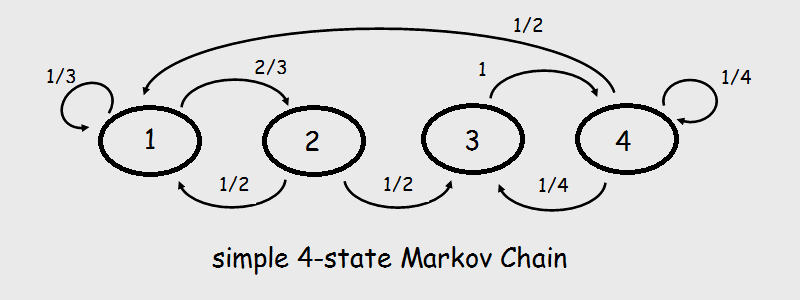
# Here is a graphical example of a simple 4-state Markov Chain, listing all of its transition probabilities:
#
# 
#
#
# ### Definition: transition matrix
#
# The _transition matrix_ is then just the matrix representation of a Markov chain's transition probabilities in the form $Q = \left[ q_{ij} \right]$in the columns, with the rows representing each possible state. Since our introductory example is for a discrete, finite space, elements of a row are the complete listing of the probability mass function for the state in question.
#
# For the example above, that'd be
#
# \begin{align}
# Q &= \begin{pmatrix}
# \frac{1}{3} & \frac{2}{3} & 0 & 0 \\
# \frac{1}{2} & 0 & \frac{1}{2} & 0 \\
# 0 & 0 & 0 & 1 \\
# \frac{1}{2} & 0 & \frac{1}{4} & \frac{1}{4} \\
# \end{pmatrix}
# \end{align}
#
# ### Usage
#
# We can use a Markov chain as a model to describe a system evolving over time. The case of $P(X_{n+1} = j | X_n = i) = q_{ij}$ only looks at the present $X_n$, ignoring events of the past. Using such a *first order* model might be too strong a starting assumption of conditional independence. We could, however, extend this model such that $P(X_{n+1} = j | X_n = i, X_{n-1} = k)$, to consider the last 2 states (second order), or even more past states.
#
# There are also such things called Markov Chain Monte Carlo, where you synthesize your own Markov Chain to let you do large-scale simulations (computer-assisted, of course).
#
# But originally, Markov came up with this idea to show there was a way to reconcile the Law of Large Numbers but relax the condition of _independent, individually distributed_, and instead of completely ignoring the past states of system, condition on the present state (first-order) to predict the future. Of course, this could be extended to condition on states prior to the present as well. He wanted to go a step beyond _i.i.d._. His experiment was with the Russian langage and its vowels and consonants, a chain of two states.
# ## Using the Transition Matrix
#
# Suppose time $n, X_n$ has distribution $\vec{s}$ ($1 \times m$ row vector). Again, in our discrete, finite state example, $\vec{s}$ is simply the PMF listed out, so its entries are non-negative and sum up to 1.0.
#
# _What is the PMF for $X_{n+1}$?_
#
# \begin{align}
# P(X_{n+1} = j) &= \sum_{i} P(X_{n+1} = j | X_n = i) \, P(X_n = i) &\quad \text{ by Law of Total Probability}\\
# &= \sum_{i}^{j} q_{ij} \, s_i &\quad \text{ definition of transition matrix; and definition of transition matrix row} \\
# &= \sum_{i}^{j} s_i \, q_{ij} &\quad \text{ but this is the } j^{th} \text{ entry of } \vec{s} \, Q
# \end{align}
#
#
# * So row vector $\vec{s} \, Q$ is the distribution at time $n+1$.
# * So row vector $\vec{s} \, Q^{2}$ is the distribution at time $n+2$ ($\vec{s}\,Q$ plays the role of $\vec{s}$).
# * So row vector $\vec{s} \, Q^{3}$ is the distribution at time $n+3$ ($\vec{s}\,Q^2$ plays the role of $\vec{s}$).
# * and so on, and so forth...
#
# Similarly, we can think about $m$ steps into the future.
#
# \begin{align}
# P(X_{n+1} = j | X_n = i) &= q_{ij} &\text{ by definition; 1 step into the future } \\
# \\\\
# P(X_{n+2} = j | X_n = i) &= \sum_k P(X_{n+2} = j | X_{n+1} = k, X_n = i) \, P(X_{n+1} = k | X_n = i) &\text{ 2 steps into the future } \\
# &= \sum_k P(X_{n+2} = j | X_{n+1} = k \require{enclose} \, \enclose{horizontalstrike}{, X_n = i}) \, P(X_{n+1} = k | X_n = i) &\text{ only the present counts } \\
# &= \sum_k q_{kj} \, q_{ik} \\
# &= \sum_k q_{ik} \, q_{kj} &\text{ but this is the } (i,j) \text{ entry of } Q^2 \\
# \\\\
# P(X_{n+m} = j | X_n = i) &= \left[ q_{i,j} \in Q^m \right]
# \end{align}
#
#
# So you see that powers of the transition matrix give us a lot of information!
# ## Stationary Distribution
#
# #### Definition
#
# $\vec{s}$ is stationary for the Markov chain we are considering if
#
# \begin{align}
# \vec{s} \, Q &= \vec{s}
# \end{align}
#
# You should immediately recognize that $\vec{s}$ is an eigenvector of transition matrix $Q$. This means that if the chain starts off in $\vec{s}$, after one step into the future it remains at $\vec{s}$. Another step into the future, and we _still_ remain at $\vec{s}$, ad nauseum. If the chain starts off with the stationary distribution, it will have that distribution forever.
#
# But that raises some questions:
#
# 1. Does a stationary distribution exist? (all elements of $\vec{s} \in \mathbb{Z}_{\ge 0}$)
# 1. Is it unique?
# 1. Does the chain converge to $\vec{s}$?
# 1. How can we compute it?
#
# It turns out, the answers to questions 1 through 3 is _yes_.
#
# Can we compute the stationary distribution _efficiently_? In certain examples of Markov chains, we can do so very easily and without using matrices!
#
# But that is the topic of the next lecture.
#
# ----
# View [Lecture 31: Markov Chains | Statistics 110](http://bit.ly/2MXMgr3) on YouTube.