#!/usr/bin/env python # coding: utf-8 # In[1]: get_ipython().run_cell_magic('html', '', '\n\n') # # Configuration # In[1]: from notebook.services.config import ConfigManager cm = ConfigManager() cm.update('livereveal', { 'theme': 'sky', 'transition': 'zoom', 'start_slideshow_at': 'selected', 'controls': True }) # In[2]: get_ipython().run_cell_magic('javascript', '', "require(['base/js/utils'],\nfunction(utils) {\n utils.load_extensions('calico-spell-check', 'calico-document-tools', 'calico-cell-tools');\n});\n") # In[3]: get_ipython().run_line_magic('load_ext', 'tikzmagic') # In[4]: get_ipython().run_cell_magic('html', '', '\n\n%load_ext tikzmagic\n') # In[1]: get_ipython().run_cell_magic('html', '', '\n\n') # # Recurrent Neural Networks # # Overview # # * Recap: Language Modeling # * Recurrent Neural Network (RNN) Language Models # * Training Problems and Solutions # - Vanishing and Exploding Gradients # - Long Short-Term Memory (LSTM) Networks # * RNNs for Sequence to Sequence Problems # * Extensions # # Language Modeling (LMs) # # A LM computes a **probability** for a **sequence of words** # # $$p(\langle w_{1}, \ldots, w_{d} \rangle)$$ # # Useful in a miriad of NLP tasks involving text generation, e.g. # - Machine Translation, # - Speech Recognition, # - Summarisation.. # # $$ # \begin{aligned} # p(\langle \text{Statistical}, \text{Natural}, \text{Language}, \text{Processing} \rangle) > \\ # p(\langle \text{Statistical}, \text{Language}, \text{Natural}, \text{Processing} \rangle) # \end{aligned} # $$ # # $n$-Gram Language Models # # In *$n$-gram language models*, the probability $p(w_{1}, \ldots, w_{d})$ of observing the sentence $(w_{1}, \ldots, w_{d})$ is **approximated** as: # # $$ # \begin{aligned} # p(w_{1}, \ldots, w_{d}) & = \prod_{i=1}^{d} p(w_{i} \mid w_{1}, \ldots, w_{i - 1}) \\ # & \approx \prod_{i=1}^{d} p(w_{i} \mid w_{i - (n - 1)}, \ldots, w_{i - 1}) \\ # & \approx \prod_{i=1}^{d} \frac{\text{count}(w_{i - (n - 1)}, \ldots, w_{i})}{\text{count}(w_{i - (n - 1)}, \ldots, w_{i - 1})} # \end{aligned} # $$ # # Example with a **bigram** ($n = 2$) **language model**: # # $$ # \begin{aligned} # p(\langle \text{Natural}, & \text{Language}, \text{Processing} \rangle) \approx \\ # & p(\text{Natural}){}\cdot{}p(\text{Language} \mid \text{Natural}) \\ # & {}\cdot{}p(\text{Processing} \mid \text{Language}) # \end{aligned} # $$ # # Recurrent Neural Networks # # * RNNs share the weights at each time step # * The output $y_{t}$ at time $t$ depends on all previous words # - $w_{t}, w_{t - 1}, \ldots, w_{1}$ # * Size scales with **number of words**, not **sequence length**! # In[9]: get_ipython().run_cell_magic('tikz', '-l arrows -s 1000,400 -sc 0.65', "\n\\newcommand{\\lstm}{\n\\definecolor{nice-red}{HTML}{E41A1C}\n\\definecolor{nice-orange}{HTML}{FF7F00}\n\\definecolor{nice-yellow}{HTML}{FFC020}\n\\definecolor{nice-green}{HTML}{4DAF4A}\n\\definecolor{nice-blue}{HTML}{377EB8}\n\\definecolor{nice-purple}{HTML}{984EA3}\n\n%lstm first step\n\n%lstm module box\n\\draw[line width=3pt, color=black!50] (0,0) rectangle (3,3);\n}\n\n\\lstm \n\\node[] at (0.5,-1.25) {$\\mathbf{x}_t$};\n\\node[] at (-1.5,2) {$\\mathbf{h}_{t-1}$};\n\\node[] at (4.25,2) {$\\mathbf{h}_t$};\n\\node[] at (2.5,5) {$\\mathbf{y}_t$};\n\n\\draw[ultra thick, ->, >=stealth'] (0.5,-0.75) -- (0.5,0);\n\\draw[ultra thick, ->, >=stealth'] (-0.75,2) -- (0,2); \n\\draw[ultra thick, ->, >=stealth'] (3,2) -- (3.75,2); \n\\draw[ultra thick, ->, >=stealth'] (2.5,3) -- (2.5,4.75); \n\n\\path[line width=3pt, ->, >=stealth', color=nice-red] (4, 2.5) edge[bend right=0, in=-110, out=-70] (-1.75, 2.5); \n \n\\node[] at (1.5,2) {$f_\\theta(\\mathbf{x}_t, \\mathbf{h}_{t-1})$};\n") #

# \begin{align} # \mathbf{h}_t &= f_{\theta}(\mathbf{x}_{t}, \mathbf{h}_{t - 1}) \\ # f_{\theta} \; & \text{is a } \textbf{transition function} \text { with parameters } \theta\\ # \theta \; & \text{can be } \textbf{learned from data}\\ # \\ # \\ # & \text{"Vanilla" Recurrent Neural Network} \\ # \mathbf{h}_t &= \text{sigmoid}(\mathbf{W}^h \mathbf{h}_{t-1}+ \mathbf{W}^x \mathbf{x}_t) # \end{align} #

# # A Recurrent Neural Network LM # # Consider the following sentence: # # $$\langle w_{1}, \ldots, w_{t - 1}, w_{t}, w_{t + 1}, \ldots, w_{d})$$ # # At each single time step $t$, the hidden state $\mathbf{h}_t$ and output $\hat{\mathbf{y}}_t$ are given by: # # $$ # \begin{aligned} # \mathbf{x}_{1} & = \text{encode}(w_{t}) \in \mathbb{R}^{d_{e}}\\ # \mathbf{h}_t & = \sigma(\mathbf{W}^h \mathbf{h}_{t-1}+ \mathbf{W}^x \mathbf{x}_t) \in \mathbb{R}^{d_{h}}\\ # \hat{\mathbf{y}}_{t} & = \text{softmax}(\mathbf{W}^o \mathbf{h}_{t}) \in \mathbb{R}^{|V|} \\ # \end{aligned} # $$ # # where $\mathbf{y}_{t} \in [0, 1]^{|V|}$ is a **probability distribution** over words in $V$. # # The probability that the $t$-th word in the sequence is $w_{j}$ is given by: # # $$p(w_{j} \mid w_{t}, \ldots, w_{1}) = \hat{\mathbf{y}}_{t, j}$$ # # Example # # Consider the word sequence $\text{encode}(\text{Natural}, \text{Language}, \text{Processing}) \rightarrow (\mathbf{x}_{1}, \mathbf{x}_{2}, \mathbf{x}_{3})$ # # Reminder: $\mathbf{h}_t = \sigma(\mathbf{W}^h \mathbf{h}_{t-1}+ \mathbf{W}^x \mathbf{x}_t + \mathbf{b})$ # # $$ # \begin{aligned} # \mathbf{h}_1 = \sigma(\mathbf{W}^h \mathbf{h}_{0} + \mathbf{W}^x \mathbf{x}_1) &\;& \hat{\mathbf{y}}_{1} = \text{softmax}(\mathbf{W}^o \mathbf{h}_{1}) \\ # \mathbf{h}_2 = \sigma(\mathbf{W}^h \mathbf{h}_{1} + \mathbf{W}^x \mathbf{x}_2) &\;& \hat{\mathbf{y}}_{2} = \text{softmax}(\mathbf{W}^o \mathbf{h}_{2}) \\ # \mathbf{h}_3 = \sigma(\mathbf{W}^h \mathbf{h}_{2} + \mathbf{W}^x \mathbf{x}_3) &\;& \hat{\mathbf{y}}_{3} = \text{softmax}(\mathbf{W}^o \mathbf{h}_{3}) \\ # \end{aligned} # $$ # # $$p(\text{Natural}, \text{Language}, \text{Processing}) = \hat{\mathbf{y}}_{1, [\text{Natural}]} \; \hat{\mathbf{y}}_{2, [\text{Language}]} \; \hat{\mathbf{y}}_{3, [\text{Processing}]}$$ # # - Initial state: $\mathbf{h}_{0} \in \mathbb{R}^{d_{h}}$, Input matrix: $\mathbf{W}^x \in \mathbb{R}^{d_{h} \times d_{x}}$ # - Transition matrix: $\mathbf{W}^h \in \mathbb{R}^{d_{h} \times d_{h}}$, Output matrix: $\mathbf{W}^o \in \mathbb{R}^{|V| \times d_{h}}$ # # Objective Function # # Recall that $\hat{\mathbf{y}}_{t} \in \mathbb{R}^{|V|}$ is a probability distribution over the vocabulary $V$. # # We can train a RNN by minimizing the **cross-entropy loss**, predicting **words** instead of classes: # # $$ # \begin{aligned} # J_{t} = - \sum_{i = 1}^{|V|} \mathbf{y}_{t, i} \log \hat{\mathbf{y}}_{t, i}, \quad \text{where} \quad \mathbf{y}_{t, i} = \left\{\begin{array}{ll}1 \; \text{if the $t$-th word is $w_{i}$,}\\0 \, \text{otherwise.}\end{array} \right. # \end{aligned} # $$ # # Evaluating Language Models # # Evaluation - negative of average log-probability over corpus: # # $$J = - \frac{1}{T} \sum_{t = 1}^{T} \sum_{j = 1}^{|V|} \mathbf{y}_{t, j} \log \hat{\mathbf{y}}_{t, j} = \frac{1}{T} J_{t}$$ # # Or also **perplexity**: # # $$PP(w_1,\ldots,w_T) = \sqrt[T]{\prod_{i = 1}^T \frac{1}{p(w_i | w_{1}, \ldots, w_{i-1})}}$$ # # Sequence-to-Sequence Models # # Recurrent Neural Networks are extremely powerful and flexible # - They can also learn to **generate** sequences # # Seq2Seq models are composed by: # - **Encoder** - Gets the input and outputs $\mathbf{v} \in \mathbb{R}^{d}$ # - **Decoder** - Gets $\mathbf{v}$ and generates the output sequence # # Seq2Seq models are widely popular in e.g.: # - *Neural Machine Translation* # - *Text Summarization* # - *Learning to Execute* # In[7]: get_ipython().run_cell_magic('tikz', '-l arrows -s 1000,400 -sc 0.65', "\n\\definecolor{nice-red}{HTML}{E41A1C}\n\\definecolor{nice-orange}{HTML}{FF7F00}\n\\definecolor{nice-yellow}{HTML}{FFC020}\n\\definecolor{nice-green}{HTML}{4DAF4A}\n\\definecolor{nice-blue}{HTML}{377EB8}\n\\definecolor{nice-purple}{HTML}{984EA3}\n\n\\newcommand{\\lstm}{\n\n%lstm first step\n\n%lstm module box\n\\draw[line width=3pt, color=black!50] (0,0) rectangle (3,3);\n \n\\draw[ultra thick, ->, >=stealth'] (0.5,-0.75) -- (0.5,0);\n\\draw[ultra thick, ->, >=stealth'] (-0.75,2) -- (0,2); \n\\draw[ultra thick, ->, >=stealth'] (3,2) -- (3.75,2); \n\\draw[ultra thick, ->, >=stealth'] (2.5,3) -- (2.5,3.75); \n}\n\n%\\lstm \n \n%\\node[] at (0.5,-1.25) {$\\mathbf{x}_t$};\n%\\node[] at (-1.5,2) {$\\mathbf{h}_{t-1}$};\n%\\node[] at (4.25,2) {$\\mathbf{h}_t$};\n%\\node[] at (2.5,5) {$\\mathbf{h}_t$}; \n%\\path[line width=3pt, ->, >=stealth', color=nice-blue] (4, 2.5) edge[bend right=0, in=-110, out=-70] (-1.75, 2.5); \n%\\node[] at (1.5,2) {$f_\\theta(\\mathbf{x}_t, \\mathbf{h}_{t-1})$};\n\n\\foreach \\x/\\w in {0/I, 1/like, 2/neural, 3/networks} {\n \\begin{scope}[shift={(\\x*3.75,0)}]\n \\lstm \n \\node[font=\\LARGE, text height=1.5ex, color=nice-red] at (0.5,-1.5) {\\bf\\w}; \n \\end{scope} \n}\n\n\\foreach \\x/\\w/\\t in {4/EOS/Ich, 5/Ich/mag, 6/mag/neuronale, 7/neuronale/Netze, 8/Netze/EOS} {\n \\begin{scope}[shift={(\\x*3.75,0)}]\n \\lstm \n \\node[font=\\LARGE, text height=1.5ex] at (0.5,-1.5) {\\bf\\w}; \n \\node[font=\\LARGE, text height=1.5ex, color=nice-blue] at (2.5,4.5) {\\bf\\t}; \n \\end{scope} \n} \n\n\\node[font=\\Huge, color=nice-red] at (16.5,1.5) {$\\mathbf{v}$}; \n") # # Problem - Training RNNs is Hard # # - **Vanishing** and **exploding** gradients [Pascanu et al. 2013]. # # Why? Multiply the same matrix $\mathbf{W}^{h}$ at each time step during forward propagation. The norm of the gradient might either tend to 0 (**vanish**) or be too large (**explode**). # # #

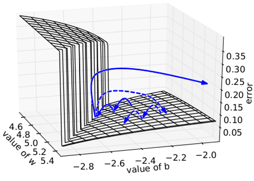
# # # Related Problem - Long-Term Dependencies # # Words from time steps far away are hardly considered when training to predict the next word. # # Example: # - John walked to the hallway. # - Mary walked in too. # - Daniel moved to the garden. # - John said "Hi" to \_\_\_\_. # # A RNN is very likely to e.g. put an uniform probability distributions over nouns in $V$, and a low probability everywhere else. # # It's an issue with language modeling, question answering, and many other tasks. # # Vanishing/Exploding Gradients - Solutions # # Several solutions in the literature: # # - Bound the gradient to a threshold (**Gradient Clipping**)
[Pascanu et al. 2013] # # - Use $\text{ReLU}(x) = \max(0, x)$ (**Re**ctified **L**inear **U**nits) or similar non-linearities instead of $\text{sigmoid}(x)$ or $\text{tanh}(x)$
[Glorot et al. 2011]. # # - Clever Initialization of the Transition Matrix ($\mathbf{W}^h = \mathbf{I}$)
[Socher et al. 2013, Le et al. 2015]. # # - Use different recurrent models that favour backpropagation
LSTM[Hochreiter et al. 1997], GRU[Chung et al. 2014]. # # Long Short-Term Memory (LSTM) Networks # # - Can adaptively learn what to **keep** (store) into memory (gate $\mathbf{i}_{t}$), **forget** (gate $\mathbf{f}_{t}$) and **output** (gate $\mathbf{o}_{t}$) # In[7]: get_ipython().run_cell_magic('tikz', '-l arrows -s 1000,400 -sc 0.65', "\n\\newcommand{\\lstm}{\n\\definecolor{nice-red}{HTML}{E41A1C}\n\\definecolor{nice-orange}{HTML}{FF7F00}\n\\definecolor{nice-yellow}{HTML}{FFC020}\n\\definecolor{nice-green}{HTML}{4DAF4A}\n\\definecolor{nice-blue}{HTML}{377EB8}\n\\definecolor{nice-purple}{HTML}{984EA3}\n\n%lstm first step\n\n%lstm module box\n\\draw[line width=3pt, color=black!50] (-6,-3) rectangle (1.5,5.25);\n\\draw[ultra thick] (0,0) rectangle (1,2);\n\n%memory ct\n\\draw[ultra thick, color=nice-purple, fill=nice-purple!10] (0,0) rectangle (1,2);\n\n%non-linearities\n\\foreach \\w/\\h/\\color in {-2/4.25/nice-blue,-2/1/nice-red,-2/-1/nice-green,0.5/-2/nice-yellow,0.5/3/black} {\n \\begin{scope}[shift={(\\w,\\h)},scale=0.5]\n \\draw[ultra thick, yshift=-0.5cm, color=\\color] plot [domain=-0.3:0.3](\\x, {(0.8/(1+exp(-15*\\x))+0.1)});\n \\draw[ultra thick, color=\\color] (0,0) circle (0.5cm);\n \\end{scope}\n}\n\n%tanh\n\\draw[thick, color=black] (0.25,3) -- (0.75,3);\n\\draw[thick, color=nice-yellow] (0.25,-2) -- (0.75,-2);\n \n \n%component-wise multiplications\n\\foreach \\w/\\h in {-1/1,0.5/-1,0.5/4.25} {\n \\begin{scope}[shift={(\\w,\\h)},scale=0.5]\n \\draw[ultra thick, color=black] (0,0) circle (0.05cm);\n \\draw[ultra thick, color=black] (0,0) circle (0.5cm);\n \\end{scope}\n}\n\n%vector concat\n\\begin{scope}[shift={(-4,1)},scale=0.5]\n \\draw[ultra thick,yshift=0.2cm] (0,0) circle (0.05cm);\n \\draw[ultra thick,yshift=-0.2cm] (0,0) circle (0.05cm);\n \\draw[ultra thick] (0,0) circle (0.5cm);\n\\end{scope}\n\n\n\\foreach \\fx/\\fy/\\tx/\\ty in {\n -5/-3.5/-5/0.85, %xt\n -5/0.85/-4.2/0.85,\n -6.5/4.25/-5/4.25, %ht1\n -5/4.25/-5/1.15,\n -5/1.15/-4.2/1.15,\n -3.75/1/-3/1, %H\n -3/4.25/-3/-2,\n -3/-2/0.25/-2, %i\n 0.5/-1.75/0.5/-1.25,\n -3/-1/-2.25/-1, %it\n -1.75/-1/0.25/-1,\n -3/1/-2.25/1, %ft\n -1.75/1/-1.25/1,\n -0.75/1/0/1,\n -3/4.25/-2.25/4.25, %ot\n -1.75/4.25/0.25/4.25,\n 0.5/2/0.5/2.75, %ct\n -5.5/2/-5.1/2, %ct1\n -5.5/2/-5.5/1,\n -6.5/1/-5.5/1,\n -4.9/2/-3.1/2,\n -2.9/2/-1/2,\n -1/2/-1/1.25 \n} {\n \\draw[ultra thick] (\\fx,\\fy) -- (\\tx,\\ty);\n}\n\n\\foreach \\fx/\\fy/\\tx/\\ty in {\n 0.5/-0.75/0.5/0, %it\n -0.75/1/0/1, %ft\n 1/1/2.25/1,\n 0.5/3.25/0.5/4,\n 0.75/4.25/2.25/4.25, %ht \n 0.5/4.5/0.5/6 \n} {\n \\draw[->, >=stealth', ultra thick] (\\fx,\\fy) -- (\\tx,\\ty);\n}\n}\n\n%\\begin{scope}[scale=0.8] \n%\\foreach \\d in {0,1} { \n%\\foreach \\t in {0,1,2,3,4} { \n%\\begin{scope}[shift={(\\t*8.5+\\d*5.5,\\d*9.5)}] \n% \\lstm\n%\\end{scope} \n%}\n%}\n%\\end{scope} \n\n \n\\lstm \n \n%annotations\n\\node[] at (-5,-3.75) {$\\mathbf{x}_t$};\n\\node[anchor=east] at (-6.5,4.25) {$\\mathbf{h}_{t-1}$};\n\\node[anchor=east] at (-6.5,1) {$\\mathbf{c}_{t-1}$};\n\\node[] at (0.5,6.25) {$\\mathbf{h}_t$};\n\\node[anchor=west] at (2.25,4.25) {$\\mathbf{h}_t$};\n\\node[anchor=west] at (2.25,1) {$\\mathbf{c}_t$}; \n\\node[xshift=0.4cm,yshift=0.25cm] at (-4,1) {$\\mathbf{H}_t$};\n\\node[xshift=0.35cm,yshift=0.25cm] at (-2,-1) {$\\mathbf{i}_t$};\n\\node[xshift=0.35cm,yshift=0.25cm] at (-2,1) {$\\mathbf{f}_t$};\n\\node[xshift=0.35cm,yshift=0.25cm] at (-2,4.25) {$\\mathbf{o}_t$}; \n \n%dummy node for left alignment\n\\node[] at (17,0) {}; \n") #

# \begin{align} # \\ # \mathbf{H}_t &= \left[ # \begin{array}{*{20}c} # \mathbf{x}_t \\ # \mathbf{h}_{t-1} # \end{array} # \right]\\ # \mathbf{i}_t &= \text{sigmoid}(\mathbf{W}^i\mathbf{H}+\mathbf{b}^i)\\ # \mathbf{f}_t &= \text{sigmoid}(\mathbf{W}^f\mathbf{H}+\mathbf{b}^f)\\ # \mathbf{o}_t &= \text{sigmoid}(\mathbf{W}^o\mathbf{H}+\mathbf{b}^o)\\ # \mathbf{c}_t &= \mathbf{f}_t \odot \mathbf{c}_{t-1} + \mathbf{i}_t \odot \tanh(\mathbf{W}^c\mathbf{H}+\mathbf{b}^c)\\ # \mathbf{h}_t &= \mathbf{o}_t \odot \tanh(\mathbf{c}_t) # \end{align} #

# # Sentence Encoding # In[8]: get_ipython().run_cell_magic('tikz', '-l arrows -s 1000,400 -sc 0.65', "\n\\newcommand{\\lstm}{\n\\definecolor{nice-red}{HTML}{E41A1C}\n\\definecolor{nice-orange}{HTML}{FF7F00}\n\\definecolor{nice-yellow}{HTML}{FFC020}\n\\definecolor{nice-green}{HTML}{4DAF4A}\n\\definecolor{nice-blue}{HTML}{377EB8}\n\\definecolor{nice-purple}{HTML}{984EA3}\n\n%lstm first step\n\n%lstm module box\n\\draw[line width=3pt, color=black!50] (-6,-3) rectangle (1.5,5.25);\n\\draw[ultra thick] (0,0) rectangle (1,2);\n\n%memory ct\n\\draw[ultra thick, color=nice-purple, fill=nice-purple!10] (0,0) rectangle (1,2);\n\n%non-linearities\n\\foreach \\w/\\h/\\color in {-2/4.25/nice-blue,-2/1/nice-red,-2/-1/nice-green,0.5/-2/nice-yellow,0.5/3/black} {\n \\begin{scope}[shift={(\\w,\\h)},scale=0.5]\n \\draw[ultra thick, yshift=-0.5cm, color=\\color] plot [domain=-0.3:0.3](\\x, {(0.8/(1+exp(-15*\\x))+0.1)});\n \\draw[ultra thick, color=\\color] (0,0) circle (0.5cm);\n \\end{scope}\n}\n\n%tanh\n\\draw[thick, color=black] (0.25,3) -- (0.75,3);\n\\draw[thick, color=nice-yellow] (0.25,-2) -- (0.75,-2);\n \n \n%component-wise multiplications\n\\foreach \\w/\\h in {-1/1,0.5/-1,0.5/4.25} {\n \\begin{scope}[shift={(\\w,\\h)},scale=0.5]\n \\draw[ultra thick, color=black] (0,0) circle (0.05cm);\n \\draw[ultra thick, color=black] (0,0) circle (0.5cm);\n \\end{scope}\n}\n\n%vector concat\n\\begin{scope}[shift={(-4,1)},scale=0.5]\n \\draw[ultra thick,yshift=0.2cm] (0,0) circle (0.05cm);\n \\draw[ultra thick,yshift=-0.2cm] (0,0) circle (0.05cm);\n \\draw[ultra thick] (0,0) circle (0.5cm);\n\\end{scope}\n\n\n\\foreach \\fx/\\fy/\\tx/\\ty in {\n -5/-3.5/-5/0.85, %xt\n -5/0.85/-4.2/0.85,\n -6.5/4.25/-5/4.25, %ht1\n -5/4.25/-5/1.15,\n -5/1.15/-4.2/1.15,\n -3.75/1/-3/1, %H\n -3/4.25/-3/-2,\n -3/-2/0.25/-2, %i\n 0.5/-1.75/0.5/-1.25,\n -3/-1/-2.25/-1, %it\n -1.75/-1/0.25/-1,\n -3/1/-2.25/1, %ft\n -1.75/1/-1.25/1,\n -0.75/1/0/1,\n -3/4.25/-2.25/4.25, %ot\n -1.75/4.25/0.25/4.25,\n 0.5/2/0.5/2.75, %ct\n -5.5/2/-5.1/2, %ct1\n -5.5/2/-5.5/1,\n -6.5/1/-5.5/1,\n -4.9/2/-3.1/2,\n -2.9/2/-1/2,\n -1/2/-1/1.25 \n} {\n \\draw[ultra thick] (\\fx,\\fy) -- (\\tx,\\ty);\n}\n\n\\foreach \\fx/\\fy/\\tx/\\ty in {\n 0.5/-0.75/0.5/0, %it\n -0.75/1/0/1, %ft\n 1/1/2.25/1,\n 0.5/3.25/0.5/4,\n 0.75/4.25/2.25/4.25, %ht \n 0.5/4.5/0.5/6 \n} {\n \\draw[->, >=stealth', ultra thick] (\\fx,\\fy) -- (\\tx,\\ty);\n}\n}\n\n\\begin{scope}[scale=0.8] \n\\foreach \\d in {0} { \n\\foreach \\t/\\word in {0/A,1/wedding,2/party,3/taking,4/pictures} { \n \\node[font=\\Huge, anchor=west] at (\\t*8.5-5.75,-4.5) {$\\mathbf{v}$\\_\\word}; \n \\begin{scope}[shift={(\\t*8.5+\\d*5.5,\\d*9.5)}] \n \\lstm \n \\end{scope} \n}\n}\n\\end{scope} \n\n\\node[font=\\Huge, anchor=west] at (27,5.75) {$\\mathbf{v}$\\_Sentence}; \n \n \n%dummy node for left alignment\n\\node[] at (17,0) {}; \n") # # Gating # In[9]: get_ipython().run_cell_magic('tikz', '-l arrows -s 1000,400 -sc 0.65', "\n\\definecolor{nice-red}{HTML}{E41A1C}\n\\definecolor{nice-orange}{HTML}{FF7F00}\n\\definecolor{nice-yellow}{HTML}{FFC020}\n\\definecolor{nice-green}{HTML}{4DAF4A}\n\\definecolor{nice-blue}{HTML}{377EB8}\n\\definecolor{nice-purple}{HTML}{984EA3}\n\n\\newcommand{\\lstm}{\n%lstm first step\n\n%lstm module box\n\\draw[line width=3pt, color=black!50] (-6,-3) rectangle (1.5,5.25);\n\\draw[ultra thick] (0,0) rectangle (1,2);\n\n%memory ct\n\\draw[ultra thick, color=nice-purple, fill=nice-purple!10] (0,0) rectangle (1,2);\n\n%non-linearities\n\\foreach \\w/\\h/\\color in {-2/4.25/nice-blue,-2/1/nice-red,-2/-1/nice-green,0.5/-2/nice-yellow,0.5/3/black} {\n \\begin{scope}[shift={(\\w,\\h)},scale=0.5]\n \\draw[ultra thick, yshift=-0.5cm, color=\\color] plot [domain=-0.3:0.3](\\x, {(0.8/(1+exp(-15*\\x))+0.1)});\n \\draw[ultra thick, color=\\color] (0,0) circle (0.5cm);\n \\end{scope}\n}\n\n%tanh\n\\draw[thick, color=black] (0.25,3) -- (0.75,3);\n\\draw[thick, color=nice-yellow] (0.25,-2) -- (0.75,-2);\n \n \n%component-wise multiplications\n\\foreach \\w/\\h in {-1/1,0.5/-1,0.5/4.25} {\n \\begin{scope}[shift={(\\w,\\h)},scale=0.5]\n \\draw[ultra thick, color=black] (0,0) circle (0.05cm);\n \\draw[ultra thick, color=black] (0,0) circle (0.5cm);\n \\end{scope}\n}\n\n%vector concat\n\\begin{scope}[shift={(-4,1)},scale=0.5]\n \\draw[ultra thick,yshift=0.2cm] (0,0) circle (0.05cm);\n \\draw[ultra thick,yshift=-0.2cm] (0,0) circle (0.05cm);\n \\draw[ultra thick] (0,0) circle (0.5cm);\n\\end{scope}\n\n\n\\foreach \\fx/\\fy/\\tx/\\ty in {\n -5/-3.5/-5/0.85, %xt\n -5/0.85/-4.2/0.85,\n -6.5/4.25/-5/4.25, %ht1\n -5/4.25/-5/1.15,\n -5/1.15/-4.2/1.15,\n -3.75/1/-3/1, %H\n -3/4.25/-3/-2,\n -3/-2/0.25/-2, %i\n 0.5/-1.75/0.5/-1.25,\n -3/-1/-2.25/-1, %it\n -1.75/-1/0.25/-1,\n -3/1/-2.25/1, %ft\n -1.75/1/-1.25/1,\n -0.75/1/0/1,\n -3/4.25/-2.25/4.25, %ot\n -1.75/4.25/0.25/4.25,\n 0.5/2/0.5/2.75, %ct\n -5.5/2/-5.1/2, %ct1\n -5.5/2/-5.5/1,\n -6.5/1/-5.5/1,\n -4.9/2/-3.1/2,\n -2.9/2/-1/2,\n -1/2/-1/1.25 \n} {\n \\draw[ultra thick] (\\fx,\\fy) -- (\\tx,\\ty);\n}\n\n\\foreach \\fx/\\fy/\\tx/\\ty in {\n 0.5/-0.75/0.5/0, %it\n -0.75/1/0/1, %ft\n 1/1/2.25/1,\n 0.5/3.25/0.5/4,\n 0.75/4.25/2.25/4.25, %ht \n 0.5/4.5/0.5/6 \n} {\n \\draw[->, >=stealth', ultra thick] (\\fx,\\fy) -- (\\tx,\\ty);\n}\n}\n\n\\begin{scope}[scale=0.8] \n\\foreach \\d in {0} { \n\\foreach \\t/\\word in {0/A,1/wedding,2/party,3/taking,4/pictures} { \n \\node[font=\\Huge, anchor=west] at (\\t*8.5-5.75,-4.5) {$\\mathbf{v}$\\_\\word}; \n \\begin{scope}[shift={(\\t*8.5+\\d*5.5,\\d*9.5)}] \n \\lstm \n \\end{scope} \n}\n}\n\\end{scope} \n\n\\node[font=\\Huge, anchor=west] at (27,5.75) {$\\mathbf{v}$\\_Sentence}; \n \n\n\\draw[line width=10pt, color=nice-red, opacity=0.8] (27.6,5) -- (27.6,0.75);\n\\draw[line width=10pt, color=nice-red, opacity=0.8] (27.5,0.75) -- (3,0.75);\n\\draw[->, >=stealth', line width=10pt, color=nice-red, opacity=0.8] (2.75,0.75) -- (2.75,-3);\n \n \n%dummy node for left alignment\n\\node[] at (17,0) {}; \n") # # Visualizing Gradients # # RNN vs. LSTM gradients on the input matrix $\mathbf{W}^x$ # # - Error is generated at 128th step and propagated back, no error from other steps. # In[10]: get_ipython().run_cell_magic('html', '', '\n\n

\n\n') # # Stacking (Deep LSTMs) # In[11]: get_ipython().run_cell_magic('tikz', '-l arrows -s 1100,500 -sc 0.65', "\n\\definecolor{nice-red}{HTML}{E41A1C}\n\\definecolor{nice-orange}{HTML}{FF7F00}\n\\definecolor{nice-yellow}{HTML}{FFC020}\n\\definecolor{nice-green}{HTML}{4DAF4A}\n\\definecolor{nice-blue}{HTML}{377EB8}\n\\definecolor{nice-purple}{HTML}{984EA3}\n\n\\newcommand{\\lstm}{\n%lstm first step\n\n%lstm module box\n\\draw[line width=3pt, color=black!50] (-6,-3) rectangle (1.5,5.25);\n\\draw[ultra thick] (0,0) rectangle (1,2);\n\n%memory ct\n\\draw[ultra thick, color=nice-purple, fill=nice-purple!10] (0,0) rectangle (1,2);\n\n%non-linearities\n\\foreach \\w/\\h/\\color in {-2/4.25/nice-blue,-2/1/nice-red,-2/-1/nice-green,0.5/-2/nice-yellow,0.5/3/black} {\n \\begin{scope}[shift={(\\w,\\h)},scale=0.5]\n \\draw[ultra thick, yshift=-0.5cm, color=\\color] plot [domain=-0.3:0.3](\\x, {(0.8/(1+exp(-15*\\x))+0.1)});\n \\draw[ultra thick, color=\\color] (0,0) circle (0.5cm);\n \\end{scope}\n}\n\n%tanh\n\\draw[thick, color=black] (0.25,3) -- (0.75,3);\n\\draw[thick, color=nice-yellow] (0.25,-2) -- (0.75,-2);\n \n \n%component-wise multiplications\n\\foreach \\w/\\h in {-1/1,0.5/-1,0.5/4.25} {\n \\begin{scope}[shift={(\\w,\\h)},scale=0.5]\n \\draw[ultra thick, color=black] (0,0) circle (0.05cm);\n \\draw[ultra thick, color=black] (0,0) circle (0.5cm);\n \\end{scope}\n}\n\n%vector concat\n\\begin{scope}[shift={(-4,1)},scale=0.5]\n \\draw[ultra thick,yshift=0.2cm] (0,0) circle (0.05cm);\n \\draw[ultra thick,yshift=-0.2cm] (0,0) circle (0.05cm);\n \\draw[ultra thick] (0,0) circle (0.5cm);\n\\end{scope}\n\n\n\\foreach \\fx/\\fy/\\tx/\\ty in {\n -5/-3.5/-5/0.85, %xt\n -5/0.85/-4.2/0.85,\n -6.5/4.25/-5/4.25, %ht1\n -5/4.25/-5/1.15,\n -5/1.15/-4.2/1.15,\n -3.75/1/-3/1, %H\n -3/4.25/-3/-2,\n -3/-2/0.25/-2, %i\n 0.5/-1.75/0.5/-1.25,\n -3/-1/-2.25/-1, %it\n -1.75/-1/0.25/-1,\n -3/1/-2.25/1, %ft\n -1.75/1/-1.25/1,\n -0.75/1/0/1,\n -3/4.25/-2.25/4.25, %ot\n -1.75/4.25/0.25/4.25,\n 0.5/2/0.5/2.75, %ct\n -5.5/2/-5.1/2, %ct1\n -5.5/2/-5.5/1,\n -6.5/1/-5.5/1,\n -4.9/2/-3.1/2,\n -2.9/2/-1/2,\n -1/2/-1/1.25 \n} {\n \\draw[ultra thick] (\\fx,\\fy) -- (\\tx,\\ty);\n}\n\n\\foreach \\fx/\\fy/\\tx/\\ty in {\n 0.5/-0.75/0.5/0, %it\n -0.75/1/0/1, %ft\n 1/1/2.25/1,\n 0.5/3.25/0.5/4,\n 0.75/4.25/2.25/4.25, %ht \n 0.5/4.5/0.5/6 \n} {\n \\draw[->, >=stealth', ultra thick] (\\fx,\\fy) -- (\\tx,\\ty);\n}\n}\n\n\\begin{scope}[scale=0.8] \n\\foreach \\d in {0,1,2} { \n\\foreach \\t/\\word in {0/A,1/wedding,2/party,3/taking,4/pictures} { \n \\node[font=\\Huge, anchor=west] at (\\t*8.5-5.75,-4.5) {$\\mathbf{v}$\\_\\word}; \n \\begin{scope}[shift={(\\t*8.5+\\d*5.5,\\d*9.5)}] \n \\lstm \n \\end{scope} \n}\n}\n\\end{scope} \n\n\\node[font=\\Huge, anchor=west] at (34,20.75) {$\\mathbf{v}$\\_Sentence}; \n\n\\draw[line width=10pt, color=nice-red, opacity=0.8] (36.4,16) -- (36.4,20); \n\\draw[line width=10pt, color=nice-red, opacity=0.8] (25.25,16) -- (36.5,16); \n\\draw[line width=10pt, color=nice-red, opacity=0.8] (25.25,8.5) -- (25.25,16); \n\\draw[line width=10pt, color=nice-red, opacity=0.8] (14,8.5) -- (25.25,8.5);\n\\draw[line width=10pt, color=nice-red, opacity=0.8] (14,8.5) -- (14,0.75);\n\\draw[line width=10pt, color=nice-red, opacity=0.8] (14,0.75) -- (3,0.75);\n\\draw[->, >=stealth', line width=10pt, color=nice-red, opacity=0.8] (2.75,0.75) -- (2.75,-3);\n \n \n%dummy node for left alignment\n\\node[] at (17,0) {}; \n") # # Applications # - Language Modeling # - Machine Translation # - Question Answering # - Dialog Modeling # - Language Generation # - Sentence Summarization # - Paraphrasing # - Sentiment Analysis # - Recognizing Textual Entailment # - ... # # Learning to Execute # # RNNs are **Turing-Complete** [Siegelman, 1995] - they can simulate arbitrary programs, given the proper parameters. # # Learning to Execute [Zaremba and Sutskever, 2014] # #

# # Implementing LSTM (TensorFlow) # ```python # lstm = rnn_cell.BasicLSTMCell(lstm_size) # # Initial state of the LSTM memory. # state = tf.zeros([batch_size, lstm.state_size]) # probabilities = [] # loss_val = 0.0 # for batch_of_words in words_in_dataset: # # State is updated after processing each batch # output, state = lstm(batch_of_words, state) # # Output is used to make next word predictions # scores = tf.matmul(output, out_w) + out_b # probabilities.append(tf.nn.softmax(scores)) # loss_val += loss(probabilities, target_words) # ``` # - Pay attention to **batching**, **bucketization** and **padding** # # Levels of Granularity # # Char-Level Language Models: Char-RNN - see e.g. [Karpathy, 2015] # # #

# # # Neural "Lego Blocks" # # We can combine models! Example: Show and Tell [Vinyals, 2015] # # #

# # # Bidirectional RNNs # # Problem - for word classification, you may need to incorporate information from both the **left** and **right** contexts of the word. # #

# #

# \begin{align} # \\ # \\ # \\ # \\ # \\ # \\ # \overleftarrow{\mathbf{h}}_t &= f_{\overleftarrow{\theta}}(\mathbf{x}_t, \overleftarrow{\mathbf{h}}_{t-1})\\ # \overrightarrow{\mathbf{h}}_t &= f_{\overrightarrow{\theta}}(\mathbf{x}_t, \overrightarrow{\mathbf{h}}_{t+1})\\ # \hat{\mathbf{y}}_t & = g(\overleftarrow{\mathbf{h}}_t, \overrightarrow{\mathbf{h}}_t) # \end{align} #

# - $\overleftarrow{\mathbf{h}}_t$ and $\overrightarrow{\mathbf{h}}_t$ represent (summarize) both the **past** and the **future** around a given sequence element. # In[ ]: