#!/usr/bin/env python
# coding: utf-8
# In[1]:
get_ipython().run_cell_magic('html', '', '\n\n\n')
# In[2]:
get_ipython().run_cell_magic('capture', '', '%load_ext autoreload\n%autoreload 2\n%matplotlib inline\nimport sys\nsys.path.append("..")\nimport statnlpbook.util as util\nimport statnlpbook.sequence as seq\nfrom statnlpbook.gmb import load_gmb_dataset\nimport pandas as pd\nimport matplotlib\nimport warnings\nwarnings.filterwarnings(\'ignore\')\nmatplotlib.rcParams[\'figure.figsize\'] = (8.0, 5.0)\nfrom collections import defaultdict, Counter\nfrom random import random\n\nfrom IPython.display import Image\n')
#
# $$
# \newcommand{\Xs}{\mathcal{X}}
# \newcommand{\Ys}{\mathcal{Y}}
# \newcommand{\y}{\mathbf{y}}
# \newcommand{\balpha}{\boldsymbol{\alpha}}
# \newcommand{\bbeta}{\boldsymbol{\beta}}
# \newcommand{\aligns}{\mathbf{a}}
# \newcommand{\align}{a}
# \newcommand{\source}{\mathbf{s}}
# \newcommand{\target}{\mathbf{t}}
# \newcommand{\ssource}{s}
# \newcommand{\starget}{t}
# \newcommand{\repr}{\mathbf{f}}
# \newcommand{\repry}{\mathbf{g}}
# \newcommand{\x}{\mathbf{x}}
# \newcommand{\prob}{p}
# \newcommand{\bar}{\,|\,}
# \newcommand{\vocab}{V}
# \newcommand{\params}{\boldsymbol{\theta}}
# \newcommand{\param}{\theta}
# \DeclareMathOperator{\perplexity}{PP}
# \DeclareMathOperator{\argmax}{argmax}
# \DeclareMathOperator{\argmin}{argmin}
# \newcommand{\train}{\mathcal{D}}
# \newcommand{\counts}[2]{\#_{#1}(#2) }
# \newcommand{\length}[1]{\text{length}(#1) }
# \newcommand{\indi}{\mathbb{I}}
# $$
# In[3]:
get_ipython().run_line_magic('load_ext', 'tikzmagic')
# # Sequence Labelling
# + POS tagging
# + Log-linear models
# + IOB encoding
# + Named entity recognition
# + Evaluating sequence labelers
# + Maximum-entropy Markov models
# + Conditional random fields
# + Beam search
# ## Sequence Labelling
#
# + Assigning exactly one label to each element in a sequence
#
# + In context of RNNs or other sequence models, example of **one-to-one** paradigm
#
#  #
#
# (In the example: Universal Semantic Tags from [Abzianidze and Bos (2017)](https://www.aclweb.org/anthology/W17-6901.pdf))
# ## Parts of speech (POS)
#
# - Group words with **similar grammatical properties**
# - [Penn Treebank](https://www.ling.upenn.edu/courses/Fall_2003/ling001/penn_treebank_pos.html) is the most commonly used POS tag set for English
# - Has 36 POS tags and 12 other tags (for punctuation and currency symbols)
# - For example, distinguishes four types of nouns and six types of verbs
#
# | | | |
# |-|-|-|
# | **NN** | noun, singular or mass | *cat, rain* |
# | **NNS** | noun, plural | *cats, tables* |
# | **NNP** | proper noun, singular | *John, IBM* |
# | **NNPS** | proper noun, plural | *Muslims, Philippines* |
#
#
# - Granularity of tags can differ
# ## Task: POS tagging
#
# Assign each word in a sentence its **part-of-speech (POS) tag**.
#
# | 1 | 2 | 3 | 4 | 5 | 6 | 7 |
# |-|-|-|-|-|-|-|
# | I | predict | that | it | will | rain | tonight |
# | PRP | VBP | IN | PRP | MD | VB | NN |
# ## Example
#
# Let's look at the [GMB (Groningen Meaning Bank) dataset](https://www.kaggle.com/shoumikgoswami/annotated-gmb-corpus/), annotated with the Penn Treebank tag set
#
# In[4]:
tokens, pos, ents = load_gmb_dataset('../data/gmb/GMB_dataset_utf8.txt')
pd.DataFrame([tokens[2], pos[2]])
# In[5]:
examples = {}
counts = Counter(tag for sent in pos for tag in sent)
words = defaultdict(set)
for x_s, y_s in zip(tokens, pos):
for i, (x, y) in enumerate(zip(x_s, y_s)):
if (y not in examples) or (random() > 0.97):
examples[y] = [x_s[j] + "/" + y_s[j] if i == j else x_s[j] for j in range(max(i-2,0),min(i+3,len(x_s)))]
words[y].add(x)
sorted_tags = sorted(counts.items(),key=lambda x:-x[1])
sorted_tags_with_examples = [(t,c,len(words[t])," ".join(examples[t])) for t,c in sorted_tags]
sorted_tags_table = pd.DataFrame(sorted_tags_with_examples, columns=['Tag','Count','Unique Tokens','Example'])
# In[6]:
sorted_tags_table[:10]
# In[33]:
plt.xticks(rotation=45, fontsize=7)
plt.bar(sorted(counts.keys(), key=counts.get), sorted(counts.values()))
# ## Sequence Labelling as Structured Prediction
#
# * Input Space $\Xs$: sequences of items to label
# * Output Space $\Ys$: sequences of output labels
# * Model: $s_{\params}(\x,\y)$
# * Prediction: $\argmax_\y s_{\params}(\x,\y)$
# ## Conditional Models
# Model probability distributions over label sequences $\y$ conditioned on input sequences $\x$
#
# $$
# s_{\params}(\x,\y) = \prob_\params(\y|\x)
# $$
#
# * Just like the conditional models from the [text classification](doc_classify_slides_short.ipynb) chapter
#
# * But the label space is *exponential* (as a function of sequence length)!
#
# * Most unique $\y$ are never even seen in training
#
# * Might be useful to **break it up**?
# ## Local Models / Classifiers
# A **fully factorised** or **local** model:
#
# $$
# p_\params(\y|\x) = \prod_{i=1}^n p_\params(y_i|\x,i,y_{1,\ldots,i-1}) \approx \prod_{i=1}^n p_\params(y_i|\x,i)
# $$
#
# * Assumption: labels are independent of each other given the input
# * Inference in this model is trivial: **greedy decoding**
# $$
# \prob_\params(\text{"PRP MD VB"} \bar \text{"it will rain"}) \approx \\\\ \prob_\params(\text{"PRP"}\bar \text{"it will rain"},1) \cdot \\ \prob_\params(\text{"MD"} \bar \text{"it will rain"},2) \cdot \\ \prob_\params(\text{"VB"} \bar \text{"it will rain"},3)
# $$
# Does this remind you of anything you've seen in previous lectures?
# $$
# \prob_\params(\text{"it will rain"}) \approx \prob_\params(\text{"it"}) \cdot \prob_\params(\text{"will"} \bar \text{"it"}) \cdot \prob_\params(\text{"rain"} \bar \text{"it will"})
# $$
# ### Graphical Representation
#
# - Models can be represented as factor graphs
# - Each variable of the model (our per-token tag labels and the input sequence $\x$) is drawn using a circle
# - *Observed* variables are shaded
# - Each factor in the model (terms in the product) is drawn as a box that connects the variables that appear in the corresponding term
# - For example, the term $p_\params(y_3|\x,3)$ would connect the variables $y_3$ and $\x$.
# In[7]:
seq.draw_local_fg(7)
# ### Parametrisation
#
# **Log-linear multiclass classifier** $p_\params(y\bar\x,i)$ to predict class for sentence $\x$ and position $i$
#
# $$
# p_\params(y\bar\x,i) \approx \frac{1}{Z_\x} \exp \langle \repr(\x,i),\params_y \rangle
# $$
#
# + $\repr(\x,i)$ is a **feature function**
# + ${Z_\x} > 0$ is a normalisation factor to ensure that $\sum_{y} p_\params(y\bar\x,i) = 1$
#
# + How far can we get with very simple features that only consider the word types (and no context)?
# Bias:
# $$
# \repr_0(\x,i) = 1
# $$
#
# Word at token to tag:
# $$
# \repr_w(\x,i) = \begin{cases}1 \text{ if }x_i=w \\\\ 0 \text{ else} \end{cases}
# $$
# In[8]:
def feat_1(x,i):
return {
'bias': 1.0,
'word:' + x[i]: 1.0,
}
train = list(zip(tokens[:-200], pos[:-200]))
dev = list(zip(tokens[-200:], pos[-200:]))
local_1 = seq.LocalSequenceLabeler(feat_1, train, class_weight='balanced')
# We can assess the accuracy of this model on the development set.
# In[9]:
seq.accuracy(dev, local_1.predict(dev))
# ### Problem 1: unknown words
#
# Many words are new, but we should still be able to tag them based on form or context:
#
# > ’Twas brillig, and the slithy toves
# Did gyre and gimble in the wabe:
# All mimsy were the borogoves,
# And the mome raths outgrabe.
#
# (Jabberwocky by Lewis Carroll)
# ### How to Improve?
#
# Look at **confusion matrix**
# In[10]:
import matplotlib.pyplot as plt
plt.rcParams['figure.figsize'] = [7, 7]
import matplotlib.pylab as plb
plb.rcParams['figure.dpi'] = 120
# In[11]:
seq.plot_confusion_matrix(dev, local_1.predict(dev), normalise=True)
# * mostly strong diagonal (good predictions)
# * `NN` receives a lot of wrong counts, often confused with `NNP`
# In[12]:
util.Carousel(local_1.errors(dev,
filter_gold=lambda y: y=='NN',
filter_guess=lambda y: y=='NNP'))
# * "walkout", "commute", "wage" are misclassified as proper nouns
# * For $f_{\text{word},w}$ feature template weights are $0$
#
# The word has not appeared in the training set!
# Proper nouns tend to be capitalised! Can we capture that with a feature?
# In[13]:
def feat_2(x,i):
return {
'bias': 1.0,
'word:' + x[i].lower(): 1.0,
'first_upper:' + str(x[i][0].isupper()): 1.0,
}
local_2 = seq.LocalSequenceLabeler(feat_2, train)
seq.accuracy(dev, local_2.predict(dev))
# Are these results actually caused by improved `NN`/`NNP` prediction?
# In[14]:
seq.plot_confusion_matrix(dev, local_2.predict(dev), normalise=True)
# In[15]:
util.Carousel(local_2.errors(dev,
filter_gold=lambda y: y=='NN',
filter_guess=lambda y: y=='NNP'))
# ### Problem 2: ambiguity
#
# *Polysemous* words or *homonyms* have multiple senses. For example, *back*:
#
# Noun:
#
# | | | | | | |
# |-|-|-|-|-|-|
# | He | is | treated | for | **back** | injury |
# | PRP | VBP | VBN | IN | **NN** | NN |
#
# Adverb:
#
# | | | | | | |
# |-|-|-|-|-|-|
# | He | is | sent | **back** | to | prison |
# | PRP | VBP | VBN | **RB** | TO | NN |
#
# Verb:
#
# | | | | | |
# |-|-|-|-|-|
# | I | can | **back** | this | up |
# | PRP | MD | **VB** | DT | RP |
# ### What other features would you try for English POS tagging?
#
#
#
#
# (In the example: Universal Semantic Tags from [Abzianidze and Bos (2017)](https://www.aclweb.org/anthology/W17-6901.pdf))
# ## Parts of speech (POS)
#
# - Group words with **similar grammatical properties**
# - [Penn Treebank](https://www.ling.upenn.edu/courses/Fall_2003/ling001/penn_treebank_pos.html) is the most commonly used POS tag set for English
# - Has 36 POS tags and 12 other tags (for punctuation and currency symbols)
# - For example, distinguishes four types of nouns and six types of verbs
#
# | | | |
# |-|-|-|
# | **NN** | noun, singular or mass | *cat, rain* |
# | **NNS** | noun, plural | *cats, tables* |
# | **NNP** | proper noun, singular | *John, IBM* |
# | **NNPS** | proper noun, plural | *Muslims, Philippines* |
#
#
# - Granularity of tags can differ
# ## Task: POS tagging
#
# Assign each word in a sentence its **part-of-speech (POS) tag**.
#
# | 1 | 2 | 3 | 4 | 5 | 6 | 7 |
# |-|-|-|-|-|-|-|
# | I | predict | that | it | will | rain | tonight |
# | PRP | VBP | IN | PRP | MD | VB | NN |
# ## Example
#
# Let's look at the [GMB (Groningen Meaning Bank) dataset](https://www.kaggle.com/shoumikgoswami/annotated-gmb-corpus/), annotated with the Penn Treebank tag set
#
# In[4]:
tokens, pos, ents = load_gmb_dataset('../data/gmb/GMB_dataset_utf8.txt')
pd.DataFrame([tokens[2], pos[2]])
# In[5]:
examples = {}
counts = Counter(tag for sent in pos for tag in sent)
words = defaultdict(set)
for x_s, y_s in zip(tokens, pos):
for i, (x, y) in enumerate(zip(x_s, y_s)):
if (y not in examples) or (random() > 0.97):
examples[y] = [x_s[j] + "/" + y_s[j] if i == j else x_s[j] for j in range(max(i-2,0),min(i+3,len(x_s)))]
words[y].add(x)
sorted_tags = sorted(counts.items(),key=lambda x:-x[1])
sorted_tags_with_examples = [(t,c,len(words[t])," ".join(examples[t])) for t,c in sorted_tags]
sorted_tags_table = pd.DataFrame(sorted_tags_with_examples, columns=['Tag','Count','Unique Tokens','Example'])
# In[6]:
sorted_tags_table[:10]
# In[33]:
plt.xticks(rotation=45, fontsize=7)
plt.bar(sorted(counts.keys(), key=counts.get), sorted(counts.values()))
# ## Sequence Labelling as Structured Prediction
#
# * Input Space $\Xs$: sequences of items to label
# * Output Space $\Ys$: sequences of output labels
# * Model: $s_{\params}(\x,\y)$
# * Prediction: $\argmax_\y s_{\params}(\x,\y)$
# ## Conditional Models
# Model probability distributions over label sequences $\y$ conditioned on input sequences $\x$
#
# $$
# s_{\params}(\x,\y) = \prob_\params(\y|\x)
# $$
#
# * Just like the conditional models from the [text classification](doc_classify_slides_short.ipynb) chapter
#
# * But the label space is *exponential* (as a function of sequence length)!
#
# * Most unique $\y$ are never even seen in training
#
# * Might be useful to **break it up**?
# ## Local Models / Classifiers
# A **fully factorised** or **local** model:
#
# $$
# p_\params(\y|\x) = \prod_{i=1}^n p_\params(y_i|\x,i,y_{1,\ldots,i-1}) \approx \prod_{i=1}^n p_\params(y_i|\x,i)
# $$
#
# * Assumption: labels are independent of each other given the input
# * Inference in this model is trivial: **greedy decoding**
# $$
# \prob_\params(\text{"PRP MD VB"} \bar \text{"it will rain"}) \approx \\\\ \prob_\params(\text{"PRP"}\bar \text{"it will rain"},1) \cdot \\ \prob_\params(\text{"MD"} \bar \text{"it will rain"},2) \cdot \\ \prob_\params(\text{"VB"} \bar \text{"it will rain"},3)
# $$
# Does this remind you of anything you've seen in previous lectures?
# $$
# \prob_\params(\text{"it will rain"}) \approx \prob_\params(\text{"it"}) \cdot \prob_\params(\text{"will"} \bar \text{"it"}) \cdot \prob_\params(\text{"rain"} \bar \text{"it will"})
# $$
# ### Graphical Representation
#
# - Models can be represented as factor graphs
# - Each variable of the model (our per-token tag labels and the input sequence $\x$) is drawn using a circle
# - *Observed* variables are shaded
# - Each factor in the model (terms in the product) is drawn as a box that connects the variables that appear in the corresponding term
# - For example, the term $p_\params(y_3|\x,3)$ would connect the variables $y_3$ and $\x$.
# In[7]:
seq.draw_local_fg(7)
# ### Parametrisation
#
# **Log-linear multiclass classifier** $p_\params(y\bar\x,i)$ to predict class for sentence $\x$ and position $i$
#
# $$
# p_\params(y\bar\x,i) \approx \frac{1}{Z_\x} \exp \langle \repr(\x,i),\params_y \rangle
# $$
#
# + $\repr(\x,i)$ is a **feature function**
# + ${Z_\x} > 0$ is a normalisation factor to ensure that $\sum_{y} p_\params(y\bar\x,i) = 1$
#
# + How far can we get with very simple features that only consider the word types (and no context)?
# Bias:
# $$
# \repr_0(\x,i) = 1
# $$
#
# Word at token to tag:
# $$
# \repr_w(\x,i) = \begin{cases}1 \text{ if }x_i=w \\\\ 0 \text{ else} \end{cases}
# $$
# In[8]:
def feat_1(x,i):
return {
'bias': 1.0,
'word:' + x[i]: 1.0,
}
train = list(zip(tokens[:-200], pos[:-200]))
dev = list(zip(tokens[-200:], pos[-200:]))
local_1 = seq.LocalSequenceLabeler(feat_1, train, class_weight='balanced')
# We can assess the accuracy of this model on the development set.
# In[9]:
seq.accuracy(dev, local_1.predict(dev))
# ### Problem 1: unknown words
#
# Many words are new, but we should still be able to tag them based on form or context:
#
# > ’Twas brillig, and the slithy toves
# Did gyre and gimble in the wabe:
# All mimsy were the borogoves,
# And the mome raths outgrabe.
#
# (Jabberwocky by Lewis Carroll)
# ### How to Improve?
#
# Look at **confusion matrix**
# In[10]:
import matplotlib.pyplot as plt
plt.rcParams['figure.figsize'] = [7, 7]
import matplotlib.pylab as plb
plb.rcParams['figure.dpi'] = 120
# In[11]:
seq.plot_confusion_matrix(dev, local_1.predict(dev), normalise=True)
# * mostly strong diagonal (good predictions)
# * `NN` receives a lot of wrong counts, often confused with `NNP`
# In[12]:
util.Carousel(local_1.errors(dev,
filter_gold=lambda y: y=='NN',
filter_guess=lambda y: y=='NNP'))
# * "walkout", "commute", "wage" are misclassified as proper nouns
# * For $f_{\text{word},w}$ feature template weights are $0$
#
# The word has not appeared in the training set!
# Proper nouns tend to be capitalised! Can we capture that with a feature?
# In[13]:
def feat_2(x,i):
return {
'bias': 1.0,
'word:' + x[i].lower(): 1.0,
'first_upper:' + str(x[i][0].isupper()): 1.0,
}
local_2 = seq.LocalSequenceLabeler(feat_2, train)
seq.accuracy(dev, local_2.predict(dev))
# Are these results actually caused by improved `NN`/`NNP` prediction?
# In[14]:
seq.plot_confusion_matrix(dev, local_2.predict(dev), normalise=True)
# In[15]:
util.Carousel(local_2.errors(dev,
filter_gold=lambda y: y=='NN',
filter_guess=lambda y: y=='NNP'))
# ### Problem 2: ambiguity
#
# *Polysemous* words or *homonyms* have multiple senses. For example, *back*:
#
# Noun:
#
# | | | | | | |
# |-|-|-|-|-|-|
# | He | is | treated | for | **back** | injury |
# | PRP | VBP | VBN | IN | **NN** | NN |
#
# Adverb:
#
# | | | | | | |
# |-|-|-|-|-|-|
# | He | is | sent | **back** | to | prison |
# | PRP | VBP | VBN | **RB** | TO | NN |
#
# Verb:
#
# | | | | | |
# |-|-|-|-|-|
# | I | can | **back** | this | up |
# | PRP | MD | **VB** | DT | RP |
# ### What other features would you try for English POS tagging?
#
#  #
# ### [ucph.page.link/pos](https://ucph.page.link/pos)
#
# ([Responses](https://docs.google.com/forms/d/1K8l0D6sTWmC4KmKJwr61zEN0eNjgUOpaDj3WSGxTuIM/edit#responses))
# ### Solution
#
# There are many possibilities:
# * last character is 's'
# * ends with -ly
# * is it after a "."
# * previous word
# * next word
#
#
# Some features we cannot use (because our local model cannot consider other tags):
# * tag of the previous words
# * tag of next word
# * whether the next word is a noun
# ## Task: Named entity recognition (NER)
#
#
# | |
# |-|
# | \[Barack Obama\]per was born in \[Hawaii\]gpe |
#
#
# per = Person
# gpe = Geopolitical Entity
# ... but this is not sequence labeling, is it?
# ## IOB encoding
#
# Label tokens as beginning (B), inside (I), or outside (O) a **named entity:**
#
# | | | | | | |
# |-|-|-|-|-|-|
# | Barack | Obama | was | born | in | Hawaii |
# | B-per | I-per | O | O | O | B-gpe |
#
# + Many tasks can be framed as sequence labelling using this idea!
# ### Named entity types in GMB dataset
#
# geo = Geographical Entity
# org = Organization
# per = Person
# gpe = Geopolitical Entity
# tim = Time indicator
# art = Artifact
# eve = Event
# nat = Natural Phenomenon
# Example sentence from GMB:
# In[16]:
pd.DataFrame([tokens[12][:11], pos[12][:11], ents[12][:11]])
# In[17]:
examples = {}
counts_ent = Counter(tag[2:] for sent in ents for tag in sent if tag.startswith("B-"))
in_entity = False
for x_s, y_s in zip(tokens, ents):
for i, (x, y) in enumerate(zip(x_s, y_s)):
if y == "O":
in_entity = False
continue
y_ent = y[2:]
if y[0] == "B":
if y_ent not in examples or random() > 0.6:
examples[y_ent] = [x]
in_entity = True
else:
in_entity = False
if y[0] == "I" and in_entity:
examples[y_ent].append(x)
sorted_ents = sorted(counts_ent.items(),key=lambda x:-x[1])
sorted_ents_with_examples = [(t,c," ".join(examples[t])) for t,c in sorted_ents]
sorted_ents_table = pd.DataFrame(sorted_ents_with_examples, columns=['Entity Type','Count','Example'])
# In[18]:
sorted_ents_table
# Can we run our simple **local model** on this?
# In[19]:
train_ner = list(zip(tokens[:-200], ents[:-200]))
dev_ner = list(zip(tokens[-200:], ents[-200:]))
def feat_2(x,i):
return {
'bias': 1.0,
'word:' + x[i].lower(): 1.0,
'first_upper:' + str(x[i][0].isupper()): 1.0,
}
local_2 = seq.LocalSequenceLabeler(feat_2, train_ner)
seq.accuracy(dev_ner, local_2.predict(dev_ner))
# This seems great, but tag distribution is also **highly skewed**:
# In[27]:
hist = Counter(tag for _, tags in dev_ner for tag in tags)
plt.bar(sorted(hist.keys(), key=hist.get), sorted(hist.values()))
# A baseline that always predicts `O` is already pretty good:
# In[20]:
only_o = [tuple(['O'] * len(tags)) for _, tags in dev_ner]
seq.accuracy(dev_ner, only_o)
# In[74]:
def get_spans(labels):
spans = []
current = [None, None, None]
for i, label in enumerate(labels):
if label.startswith("I-") and label[2:] == current[0]:
# continued span
continue
# push span, if there is any
if current[0] is not None:
current[2] = i
spans.append(current)
current = [None, None, None]
if label.startswith("B-"):
current[0] = label[2:]
current[1] = i
if current[0] is not None:
current[2] = len(labels)
spans.append(current)
return spans
def _calculate_prf(preds, golds):
total_pred, total_gold, match = 0, 0, 0
for pred, gold in zip(preds, golds):
pred_s = get_spans(pred)
gold_s = get_spans(gold)
total_pred += len(pred_s)
total_gold += len(gold_s)
match += sum(s in pred_s for s in gold_s)
# precision: % of entities found by the system that are correct
p = match / total_pred if total_pred else 0.0
# recall: % of entities in dataset found by the system
r = match / total_gold if total_gold else 0.0
# f-score: harmonic mean of precision and recall
f = 2 * (p * r) / (p + r) if p + r else 0.0
return p, r, f
def print_prf(goldset, preds):
p, r, f = _calculate_prf(preds, [s[1] for s in goldset])
print(f"precision: {p:.2f}\nrecall: {r:.2f}\nf-score: {f:.2f}")
# Tasks like NER are more commonly evaluated with...
#
# ### Precision, recall, and F-score
#
# \begin{align}
# \text{precision} & = \frac{|\text{predicted}\cap\text{annotated}|}{|\text{predicted}|} \\[.5em]
# \text{recall} & = \frac{|\text{predicted}\cap\text{annotated}|}{|\text{annotated}|} \\[.5em]
# F & = 2 \cdot \frac{\text{precision}\cdot\text{recall}}{\text{precision}+\text{recall}} \\
# \end{align}
#
# Example:
# In[86]:
pd.DataFrame([dev_ner[18][0], dev_ner[18][1], local_2_pred_dev[18]])
# predicted = {2004, Iraq}
#
# annotated = {2004, southern Iraq}
# In[87]:
print_prf([dev_ner[18]], [local_2_pred_dev[18]])
# back to the full dev set...
# In[50]:
local_2_pred_dev = local_2.predict(dev_ner)
print_prf(dev_ner, local_2_pred_dev)
# In[46]:
print_prf(dev_ner, only_o)
# ## Sequence labelling with neural networks
# We can use BiLSTMs for that!
#
#
#
#
# ### [ucph.page.link/pos](https://ucph.page.link/pos)
#
# ([Responses](https://docs.google.com/forms/d/1K8l0D6sTWmC4KmKJwr61zEN0eNjgUOpaDj3WSGxTuIM/edit#responses))
# ### Solution
#
# There are many possibilities:
# * last character is 's'
# * ends with -ly
# * is it after a "."
# * previous word
# * next word
#
#
# Some features we cannot use (because our local model cannot consider other tags):
# * tag of the previous words
# * tag of next word
# * whether the next word is a noun
# ## Task: Named entity recognition (NER)
#
#
# | |
# |-|
# | \[Barack Obama\]per was born in \[Hawaii\]gpe |
#
#
# per = Person
# gpe = Geopolitical Entity
# ... but this is not sequence labeling, is it?
# ## IOB encoding
#
# Label tokens as beginning (B), inside (I), or outside (O) a **named entity:**
#
# | | | | | | |
# |-|-|-|-|-|-|
# | Barack | Obama | was | born | in | Hawaii |
# | B-per | I-per | O | O | O | B-gpe |
#
# + Many tasks can be framed as sequence labelling using this idea!
# ### Named entity types in GMB dataset
#
# geo = Geographical Entity
# org = Organization
# per = Person
# gpe = Geopolitical Entity
# tim = Time indicator
# art = Artifact
# eve = Event
# nat = Natural Phenomenon
# Example sentence from GMB:
# In[16]:
pd.DataFrame([tokens[12][:11], pos[12][:11], ents[12][:11]])
# In[17]:
examples = {}
counts_ent = Counter(tag[2:] for sent in ents for tag in sent if tag.startswith("B-"))
in_entity = False
for x_s, y_s in zip(tokens, ents):
for i, (x, y) in enumerate(zip(x_s, y_s)):
if y == "O":
in_entity = False
continue
y_ent = y[2:]
if y[0] == "B":
if y_ent not in examples or random() > 0.6:
examples[y_ent] = [x]
in_entity = True
else:
in_entity = False
if y[0] == "I" and in_entity:
examples[y_ent].append(x)
sorted_ents = sorted(counts_ent.items(),key=lambda x:-x[1])
sorted_ents_with_examples = [(t,c," ".join(examples[t])) for t,c in sorted_ents]
sorted_ents_table = pd.DataFrame(sorted_ents_with_examples, columns=['Entity Type','Count','Example'])
# In[18]:
sorted_ents_table
# Can we run our simple **local model** on this?
# In[19]:
train_ner = list(zip(tokens[:-200], ents[:-200]))
dev_ner = list(zip(tokens[-200:], ents[-200:]))
def feat_2(x,i):
return {
'bias': 1.0,
'word:' + x[i].lower(): 1.0,
'first_upper:' + str(x[i][0].isupper()): 1.0,
}
local_2 = seq.LocalSequenceLabeler(feat_2, train_ner)
seq.accuracy(dev_ner, local_2.predict(dev_ner))
# This seems great, but tag distribution is also **highly skewed**:
# In[27]:
hist = Counter(tag for _, tags in dev_ner for tag in tags)
plt.bar(sorted(hist.keys(), key=hist.get), sorted(hist.values()))
# A baseline that always predicts `O` is already pretty good:
# In[20]:
only_o = [tuple(['O'] * len(tags)) for _, tags in dev_ner]
seq.accuracy(dev_ner, only_o)
# In[74]:
def get_spans(labels):
spans = []
current = [None, None, None]
for i, label in enumerate(labels):
if label.startswith("I-") and label[2:] == current[0]:
# continued span
continue
# push span, if there is any
if current[0] is not None:
current[2] = i
spans.append(current)
current = [None, None, None]
if label.startswith("B-"):
current[0] = label[2:]
current[1] = i
if current[0] is not None:
current[2] = len(labels)
spans.append(current)
return spans
def _calculate_prf(preds, golds):
total_pred, total_gold, match = 0, 0, 0
for pred, gold in zip(preds, golds):
pred_s = get_spans(pred)
gold_s = get_spans(gold)
total_pred += len(pred_s)
total_gold += len(gold_s)
match += sum(s in pred_s for s in gold_s)
# precision: % of entities found by the system that are correct
p = match / total_pred if total_pred else 0.0
# recall: % of entities in dataset found by the system
r = match / total_gold if total_gold else 0.0
# f-score: harmonic mean of precision and recall
f = 2 * (p * r) / (p + r) if p + r else 0.0
return p, r, f
def print_prf(goldset, preds):
p, r, f = _calculate_prf(preds, [s[1] for s in goldset])
print(f"precision: {p:.2f}\nrecall: {r:.2f}\nf-score: {f:.2f}")
# Tasks like NER are more commonly evaluated with...
#
# ### Precision, recall, and F-score
#
# \begin{align}
# \text{precision} & = \frac{|\text{predicted}\cap\text{annotated}|}{|\text{predicted}|} \\[.5em]
# \text{recall} & = \frac{|\text{predicted}\cap\text{annotated}|}{|\text{annotated}|} \\[.5em]
# F & = 2 \cdot \frac{\text{precision}\cdot\text{recall}}{\text{precision}+\text{recall}} \\
# \end{align}
#
# Example:
# In[86]:
pd.DataFrame([dev_ner[18][0], dev_ner[18][1], local_2_pred_dev[18]])
# predicted = {2004, Iraq}
#
# annotated = {2004, southern Iraq}
# In[87]:
print_prf([dev_ner[18]], [local_2_pred_dev[18]])
# back to the full dev set...
# In[50]:
local_2_pred_dev = local_2.predict(dev_ner)
print_prf(dev_ner, local_2_pred_dev)
# In[46]:
print_prf(dev_ner, only_o)
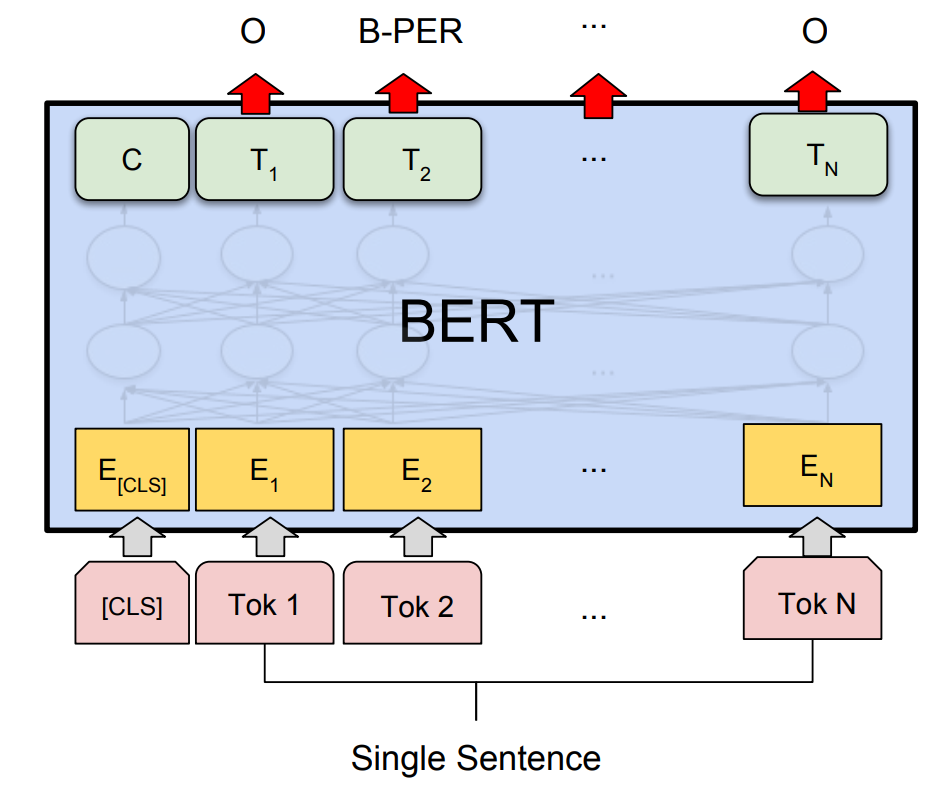
# ## Sequence labelling with neural networks
# We can use BiLSTMs for that!
#
#
#  #
#
# Source: https://guillaumegenthial.github.io/sequence-tagging-with-tensorflow.html
# ### Reminder
# A recurrent neural network (plain RNN, LSTM, GRU, ...) computes its output based on a hidden, internal state:
#
# $$
# {\mathbf{y}}_{t} = \text{RNN}(\x_t, {\mathbf{h}}_{t})
# $$
#
#
# A **bi-directional** RNN is just two uni-directional RNNs combined:
#
# \begin{align}
# \overrightarrow{\mathbf{y}_{t}} & = \overrightarrow{\text{RNN}}(\x_t, \overrightarrow{\mathbf{h}_{t}})\\
# \overleftarrow{\mathbf{y}_{t}} & = \overleftarrow{\text{RNN}}(\x_t, \overleftarrow{\mathbf{h}_{t}})
# \\
# {\mathbf{y}}_{t} & = \overrightarrow{\mathbf{y}_{t}} \oplus \overleftarrow{\mathbf{y}_{t}} \\
# \end{align}
#
# To predict label probabilities, we use the **softmax function**:
#
#
# $$
# \begin{aligned}
# {\mathbf{y}}_{t} & = \overrightarrow{\mathbf{y}_{t}} \oplus \overleftarrow{\mathbf{y}_{t}} \\
# \hat{\mathbf{y}}_{t} & = \text{softmax}(\mathbf{W}^o \mathbf{y}_{t}) \in \mathbb{R}^{|V|} \\
# \end{aligned}
# $$
#
# We can also use transformers such as BERT
# 
# ### Note on tokenisation
#
# Parts of speech are defined for *words*.
#
# Tagger must output one tag per word even if using other tokenisation internally.
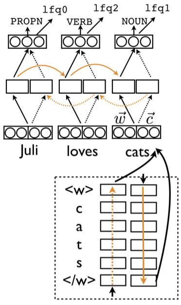
# ### Tokenisation
# Combining word representations with character representations improves POS tagging:
#
#
#
#
#
# Source: https://guillaumegenthial.github.io/sequence-tagging-with-tensorflow.html
# ### Reminder
# A recurrent neural network (plain RNN, LSTM, GRU, ...) computes its output based on a hidden, internal state:
#
# $$
# {\mathbf{y}}_{t} = \text{RNN}(\x_t, {\mathbf{h}}_{t})
# $$
#
#
# A **bi-directional** RNN is just two uni-directional RNNs combined:
#
# \begin{align}
# \overrightarrow{\mathbf{y}_{t}} & = \overrightarrow{\text{RNN}}(\x_t, \overrightarrow{\mathbf{h}_{t}})\\
# \overleftarrow{\mathbf{y}_{t}} & = \overleftarrow{\text{RNN}}(\x_t, \overleftarrow{\mathbf{h}_{t}})
# \\
# {\mathbf{y}}_{t} & = \overrightarrow{\mathbf{y}_{t}} \oplus \overleftarrow{\mathbf{y}_{t}} \\
# \end{align}
#
# To predict label probabilities, we use the **softmax function**:
#
#
# $$
# \begin{aligned}
# {\mathbf{y}}_{t} & = \overrightarrow{\mathbf{y}_{t}} \oplus \overleftarrow{\mathbf{y}_{t}} \\
# \hat{\mathbf{y}}_{t} & = \text{softmax}(\mathbf{W}^o \mathbf{y}_{t}) \in \mathbb{R}^{|V|} \\
# \end{aligned}
# $$
#
# We can also use transformers such as BERT
# 
# ### Note on tokenisation
#
# Parts of speech are defined for *words*.
#
# Tagger must output one tag per word even if using other tokenisation internally.
# ### Tokenisation
# Combining word representations with character representations improves POS tagging:
#
#
#  #
#
# ([Plank et al., 2016](https://aclanthology.org/P16-2067/))
# ### An important technical detail
#
# The linear transformation $\mathbf{W}^o \mathbf{y}_{t}$ is usually not modelled as part of the RNN itself in most deep learning frameworks.
#
# Instead, look for one of
#
# + **feed-forward layer**
# + **dense layer** (*e.g. in Keras*)
# + **linear layer** (*e.g. in PyTorch*)
#
# with a softmax activation
# ### Is it all the same?
#
# Remember the log-linear classifier:
#
# $$
# p_\params(y\bar\x,i) = \frac{1}{Z_\x} \exp \langle \repr(\x,i),\params_y \rangle
# $$
#
# A neural sequence model with a softmax layer on top is also modelling $p_\params(y\bar\x,i)$
#
# So if you take $\params$ to be the set of parameters of the neural network, then:
#
# \begin{align}
# \hat{\mathbf{y}}_{t} & = \text{softmax}(\hat{\mathbf{h}}_{t}) \\
# &= \frac{1}{Z_\x} \exp \langle \hat{\mathbf{h}}_{t},\params_y \rangle \\
# \end{align}
# ### What is the difference?
#
#
#
# ### [ucph.page.link/seq](https://ucph.page.link/seq)
#
# ([Responses](https://docs.google.com/forms/d/1X6LKsQ3a9_XcsZm5gpa8p-q9brXosjlbTubp2nqR1pk/edit#responses))
# ### Solution
#
# * Incorrect: That neural sequence models can use context: log-linear models can too
# * Correct: That neural sequence models have more parameters (generally)
# * Incorrect: That neural sequence models are global (not local) models (both can be either local or global)
# * Correct: That neural sequence models learn features on their own
# * Correct: That log-linear models can only combine features linearly
# * Incorrect: That log-linear models perform greedy inference
# * Incorrect: That log-linear models can only use the left context (preceding tokens)
# What haven't we modelled yet?
# ## There are *dependencies* between consecutive labels!
# Can you think about fitting words for this POS tag sequence?
#
# | | | |
# |-|-|-|
# | DT | JJ | NN |
# | *determiner* | *adjective* | *noun (singular or mass)* |
# What about this one?
#
# | | |
# |-|-|
# | DT | VB |
# | *determiner* | *verb (base form)* |
# + After determiners (`DT`), adjectives and nouns are much more likely than verbs
# + *Local* models cannot *directly* capture this
# In[19]:
util.Carousel(local_2.errors(dev_ner,
filter_guess=lambda y: y.startswith("I-"),
filter_gold=lambda y: y.startswith("B-")))
# In the IOB tagging scheme:
#
# + `I-[label]` can logically **only** appear after `B-[label]`!
#
# The following can **never** be valid tag sequences:
#
# * `O I-per`
#
# * `B-per I-geo`
#
# Remember that
#
# $$
# p_\params(\y|\x) = \prod_{i=1}^n p_\params(y_i|\x,i,y_{1,\ldots,i-1})
# $$
#
# What if we went from this...
#
# $$
# \approx \prod_{i=1}^n p_\params(y_i|\x,i)
# $$
#
# ...to this?
#
# $$
# \approx \prod_{i=1}^n p_\params(y_i|\x,\color{red}{y_{i-1}},i)
# $$
#
# Does this remind you of anything you've seen in previous lectures?
# ### First-order Markov assumption
#
# * Probability of a label depends only on (the input and) the previous label
#
# ### Example
#
# $$
# \prob_\params(\text{"O I-per I-per"} \bar \text{"president Bill Clinton"}) = \\
# \prob_\params(\text{"O"}\bar \text{"president Bill Clinton"},\text{""},1) ~ \cdot \\
# \prob_\params(\text{"I-per"} \bar \text{"president Bill Clinton"},\text{"O"},2) ~ \cdot \\
# \prob_\params(\text{"I-per"} \bar \text{"president Bill Clinton"},\text{"I-per"},3) \\
# $$
# ## Maximum Entropy Markov Models (MEMM)
#
# Log-linear version with access to previous label:
#
# $$
# p_\params(y_i|\x,y_{i-1},i) = \frac{1}{Z_{\x,y_{i-1},i}} \exp \langle \repr(\x,y_{i-1},i),\params_{y_i} \rangle
# $$
#
# where
# $$Z_{\x,y_{i-1},i}=\sum_y \exp \langle \repr(\x,y_{i-1},i),\params_{y_i} \rangle$$
# is a *local* per-token normalisation factor.
# ### Graphical Representation
#
# - Reminder: models can be represented as factor graphs
# - Each variable of the model (our per-token tag labels and the input sequence $\x$) is drawn using a circle
# - As before, *observed* variables are shaded
# - Each factor in the model (terms in the product) is drawn as a box that connects the variables that appear in the corresponding term
# In[20]:
seq.draw_transition_fg(7)
# ### Training MEMMs
# Optimising the conditional log-likelihood
#
# $$
# \sum_{(\x,\y) \in \train} \log \prob_\params(\y|\x)
# $$
# Decomposes nicely:
# $$
# \sum_{(\x,\y) \in \train} \sum_{i=1}^{|\x|} \log \prob_\params(y_i|\x,y_{i-1},i)
# $$
# Easy to train
# * Equivalent to a **logistic regression objective** for a classifier that assigns labels based on previous gold labels
# However...
#
# ### Local normalisation introduces *label bias*
#
# + Tag probabilities always sum to 1 at each position
# + Can lead to MEMMs effectively "ignoring" the inputs
# ## Conditional Random Fields (CRF)
#
# Replace *local* with *global* normalisation.
#
# Instead of normalising across all possible next states $y_{i+1}$ given a current state $y_i$ and observation $\x$,
#
# the CRF normalises across all possible *sequences* $\y$ given observation $\x$.
# Formally:
#
# $$
# p_\params(y_i|\x,y_{i-1},i) = \frac{1}{Z_{\x}} \exp \langle \repr(\x,y_{i-1},i),\params_{y_i} \rangle
# $$
#
# where
# $$Z_{\x}=\sum_\y \prod_i^{|\x|} \exp \langle \repr(\x,y_{i-1},i), \params_{y_i} \rangle$$
# is a *global* normalisation constant depending on $\x$.
#
# Notably, each term $\exp \langle \repr(\x,y_{i-1},i), \params_{y_i} \rangle$ in the product can now take on values in $[0,\infty)$ as opposed to the MEMM terms in $[0,1]$.
# ***
#
# + More precisely, this is a **linear-chain CRF**.
#
# (CRFs can be applied to any graph structure, but we are only considering sequences.)
#
# ## Pros and cons of CRFs
#
#
# ### 👍
#
# + Finds globally optimal label sequence
# + Eliminates label bias
#
# ### 👎
#
# + More difficult to train (—cannot break down into local terms anymore!)
# The best of both worlds?
#
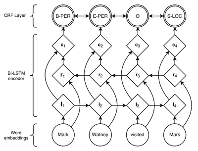
# ## Neural CRF
#
# + We can **combine** our neural sequence models with a CRF!
#
#
# $$
# p_\params(y_i|\x,y_{i-1},i) = \frac{1}{Z_{\x}} \exp \langle \hat{\mathbf{h}}_{t},\params_{y_i} \rangle
# $$
#
# 
#
# (from [Lample et al., 2016](https://www.aclweb.org/anthology/N16-1030))
# ## Prediction in MEMMs, CRFs, neural CRFs, ...
#
# To predict the best label sequence, find a $\y^*$ with maximal conditional probability
#
# $$
# \y^* =\argmax_\y \prob_\params(\y|\x).
# $$
# ## Greedy Prediction
#
# Simplest option:
# * Choose highest scoring label for token 1
# * Choose highest scoring label for token 2, conditioned on best label from 1
# * etc.
# But...
#
# + May lead to **search errors** when returned $\y^*$ is not highest scoring **global** solution
# ### Problem
#
# We cannot simply choose each label in isolation because **decisions depend on each other.**
# ## Beam Search
#
# Keep a "beam" of the best $\beta$ previous solutions
#
# 1. Choose $\beta$ highest scoring labels for token 1
# 2. 1. For each of the previous $\beta$ labels: predict probabilities for next label, conditioned on the previous label(s)
# 2. **Sum** the log-likelihoods for previous states and next label
# 3. **Prune** the beam by only keeping the top $\beta$ paths
# 3. Repeat until end of sequence
# ## Summary
#
#
# - Many problems can be cast as sequence labelling
# - POS tagging
# - Named entity recognition (with IOB encoding)
#
# - Models are similar to sequence **classifiers** but are sequential
# - Log-linear models rely on good feature engineering
# - Neural sequence labelers rely on substantial amounts of training data but generally perform better
#
# - CRFs model label dependencies
# - Can be stacked on top of neural networks
# - Exact inference is expensive
# - ...but greedy and beam search often work well
#
# ## Background Material
#
# - Longer introduction to sequence labelling with linear chain models: [notes](chapters/sequence_labeling.ipynb)
# - Longer introduction to sequence labelling with CRFs: [slides](chapters/sequence_labeling_crf_slides.ipynb)
# - Jurafsky & Martin, Speech and Language Processing, [§8.4 and §8.5](https://web.stanford.edu/~jurafsky/slp3/8.pdf) introduces Markov chains, HMMs, & MEMMs
# - Tutorial on CRFs: Sutton & McCallum, [An Introduction to Conditional Random Fields for Relational Learning](https://people.cs.umass.edu/~mccallum/papers/crf-tutorial.pdf)
# - LSTM-CRF architecture: [Huang et al., Bidirectional LSTM-CRF for Sequence Tagging](https://arxiv.org/pdf/1508.01991v1.pdf)
# - Globally Normalized Transition-Based Neural Networks: [Andor et al., 2016](https://arxiv.org/abs/1603.06042)
#
#
# ([Plank et al., 2016](https://aclanthology.org/P16-2067/))
# ### An important technical detail
#
# The linear transformation $\mathbf{W}^o \mathbf{y}_{t}$ is usually not modelled as part of the RNN itself in most deep learning frameworks.
#
# Instead, look for one of
#
# + **feed-forward layer**
# + **dense layer** (*e.g. in Keras*)
# + **linear layer** (*e.g. in PyTorch*)
#
# with a softmax activation
# ### Is it all the same?
#
# Remember the log-linear classifier:
#
# $$
# p_\params(y\bar\x,i) = \frac{1}{Z_\x} \exp \langle \repr(\x,i),\params_y \rangle
# $$
#
# A neural sequence model with a softmax layer on top is also modelling $p_\params(y\bar\x,i)$
#
# So if you take $\params$ to be the set of parameters of the neural network, then:
#
# \begin{align}
# \hat{\mathbf{y}}_{t} & = \text{softmax}(\hat{\mathbf{h}}_{t}) \\
# &= \frac{1}{Z_\x} \exp \langle \hat{\mathbf{h}}_{t},\params_y \rangle \\
# \end{align}
# ### What is the difference?
#
#
#
# ### [ucph.page.link/seq](https://ucph.page.link/seq)
#
# ([Responses](https://docs.google.com/forms/d/1X6LKsQ3a9_XcsZm5gpa8p-q9brXosjlbTubp2nqR1pk/edit#responses))
# ### Solution
#
# * Incorrect: That neural sequence models can use context: log-linear models can too
# * Correct: That neural sequence models have more parameters (generally)
# * Incorrect: That neural sequence models are global (not local) models (both can be either local or global)
# * Correct: That neural sequence models learn features on their own
# * Correct: That log-linear models can only combine features linearly
# * Incorrect: That log-linear models perform greedy inference
# * Incorrect: That log-linear models can only use the left context (preceding tokens)
# What haven't we modelled yet?
# ## There are *dependencies* between consecutive labels!
# Can you think about fitting words for this POS tag sequence?
#
# | | | |
# |-|-|-|
# | DT | JJ | NN |
# | *determiner* | *adjective* | *noun (singular or mass)* |
# What about this one?
#
# | | |
# |-|-|
# | DT | VB |
# | *determiner* | *verb (base form)* |
# + After determiners (`DT`), adjectives and nouns are much more likely than verbs
# + *Local* models cannot *directly* capture this
# In[19]:
util.Carousel(local_2.errors(dev_ner,
filter_guess=lambda y: y.startswith("I-"),
filter_gold=lambda y: y.startswith("B-")))
# In the IOB tagging scheme:
#
# + `I-[label]` can logically **only** appear after `B-[label]`!
#
# The following can **never** be valid tag sequences:
#
# * `O I-per`
#
# * `B-per I-geo`
#
# Remember that
#
# $$
# p_\params(\y|\x) = \prod_{i=1}^n p_\params(y_i|\x,i,y_{1,\ldots,i-1})
# $$
#
# What if we went from this...
#
# $$
# \approx \prod_{i=1}^n p_\params(y_i|\x,i)
# $$
#
# ...to this?
#
# $$
# \approx \prod_{i=1}^n p_\params(y_i|\x,\color{red}{y_{i-1}},i)
# $$
#
# Does this remind you of anything you've seen in previous lectures?
# ### First-order Markov assumption
#
# * Probability of a label depends only on (the input and) the previous label
#
# ### Example
#
# $$
# \prob_\params(\text{"O I-per I-per"} \bar \text{"president Bill Clinton"}) = \\
# \prob_\params(\text{"O"}\bar \text{"president Bill Clinton"},\text{""},1) ~ \cdot \\
# \prob_\params(\text{"I-per"} \bar \text{"president Bill Clinton"},\text{"O"},2) ~ \cdot \\
# \prob_\params(\text{"I-per"} \bar \text{"president Bill Clinton"},\text{"I-per"},3) \\
# $$
# ## Maximum Entropy Markov Models (MEMM)
#
# Log-linear version with access to previous label:
#
# $$
# p_\params(y_i|\x,y_{i-1},i) = \frac{1}{Z_{\x,y_{i-1},i}} \exp \langle \repr(\x,y_{i-1},i),\params_{y_i} \rangle
# $$
#
# where
# $$Z_{\x,y_{i-1},i}=\sum_y \exp \langle \repr(\x,y_{i-1},i),\params_{y_i} \rangle$$
# is a *local* per-token normalisation factor.
# ### Graphical Representation
#
# - Reminder: models can be represented as factor graphs
# - Each variable of the model (our per-token tag labels and the input sequence $\x$) is drawn using a circle
# - As before, *observed* variables are shaded
# - Each factor in the model (terms in the product) is drawn as a box that connects the variables that appear in the corresponding term
# In[20]:
seq.draw_transition_fg(7)
# ### Training MEMMs
# Optimising the conditional log-likelihood
#
# $$
# \sum_{(\x,\y) \in \train} \log \prob_\params(\y|\x)
# $$
# Decomposes nicely:
# $$
# \sum_{(\x,\y) \in \train} \sum_{i=1}^{|\x|} \log \prob_\params(y_i|\x,y_{i-1},i)
# $$
# Easy to train
# * Equivalent to a **logistic regression objective** for a classifier that assigns labels based on previous gold labels
# However...
#
# ### Local normalisation introduces *label bias*
#
# + Tag probabilities always sum to 1 at each position
# + Can lead to MEMMs effectively "ignoring" the inputs
# ## Conditional Random Fields (CRF)
#
# Replace *local* with *global* normalisation.
#
# Instead of normalising across all possible next states $y_{i+1}$ given a current state $y_i$ and observation $\x$,
#
# the CRF normalises across all possible *sequences* $\y$ given observation $\x$.
# Formally:
#
# $$
# p_\params(y_i|\x,y_{i-1},i) = \frac{1}{Z_{\x}} \exp \langle \repr(\x,y_{i-1},i),\params_{y_i} \rangle
# $$
#
# where
# $$Z_{\x}=\sum_\y \prod_i^{|\x|} \exp \langle \repr(\x,y_{i-1},i), \params_{y_i} \rangle$$
# is a *global* normalisation constant depending on $\x$.
#
# Notably, each term $\exp \langle \repr(\x,y_{i-1},i), \params_{y_i} \rangle$ in the product can now take on values in $[0,\infty)$ as opposed to the MEMM terms in $[0,1]$.
# ***
#
# + More precisely, this is a **linear-chain CRF**.
#
# (CRFs can be applied to any graph structure, but we are only considering sequences.)
#
# ## Pros and cons of CRFs
#
#
# ### 👍
#
# + Finds globally optimal label sequence
# + Eliminates label bias
#
# ### 👎
#
# + More difficult to train (—cannot break down into local terms anymore!)
# The best of both worlds?
#
# ## Neural CRF
#
# + We can **combine** our neural sequence models with a CRF!
#
#
# $$
# p_\params(y_i|\x,y_{i-1},i) = \frac{1}{Z_{\x}} \exp \langle \hat{\mathbf{h}}_{t},\params_{y_i} \rangle
# $$
#
# 
#
# (from [Lample et al., 2016](https://www.aclweb.org/anthology/N16-1030))
# ## Prediction in MEMMs, CRFs, neural CRFs, ...
#
# To predict the best label sequence, find a $\y^*$ with maximal conditional probability
#
# $$
# \y^* =\argmax_\y \prob_\params(\y|\x).
# $$
# ## Greedy Prediction
#
# Simplest option:
# * Choose highest scoring label for token 1
# * Choose highest scoring label for token 2, conditioned on best label from 1
# * etc.
# But...
#
# + May lead to **search errors** when returned $\y^*$ is not highest scoring **global** solution
# ### Problem
#
# We cannot simply choose each label in isolation because **decisions depend on each other.**
# ## Beam Search
#
# Keep a "beam" of the best $\beta$ previous solutions
#
# 1. Choose $\beta$ highest scoring labels for token 1
# 2. 1. For each of the previous $\beta$ labels: predict probabilities for next label, conditioned on the previous label(s)
# 2. **Sum** the log-likelihoods for previous states and next label
# 3. **Prune** the beam by only keeping the top $\beta$ paths
# 3. Repeat until end of sequence
# ## Summary
#
#
# - Many problems can be cast as sequence labelling
# - POS tagging
# - Named entity recognition (with IOB encoding)
#
# - Models are similar to sequence **classifiers** but are sequential
# - Log-linear models rely on good feature engineering
# - Neural sequence labelers rely on substantial amounts of training data but generally perform better
#
# - CRFs model label dependencies
# - Can be stacked on top of neural networks
# - Exact inference is expensive
# - ...but greedy and beam search often work well
#
# ## Background Material
#
# - Longer introduction to sequence labelling with linear chain models: [notes](chapters/sequence_labeling.ipynb)
# - Longer introduction to sequence labelling with CRFs: [slides](chapters/sequence_labeling_crf_slides.ipynb)
# - Jurafsky & Martin, Speech and Language Processing, [§8.4 and §8.5](https://web.stanford.edu/~jurafsky/slp3/8.pdf) introduces Markov chains, HMMs, & MEMMs
# - Tutorial on CRFs: Sutton & McCallum, [An Introduction to Conditional Random Fields for Relational Learning](https://people.cs.umass.edu/~mccallum/papers/crf-tutorial.pdf)
# - LSTM-CRF architecture: [Huang et al., Bidirectional LSTM-CRF for Sequence Tagging](https://arxiv.org/pdf/1508.01991v1.pdf)
# - Globally Normalized Transition-Based Neural Networks: [Andor et al., 2016](https://arxiv.org/abs/1603.06042)