#!/usr/bin/env python # coding: utf-8 # # Free body diagram # # Marcos Duarte #

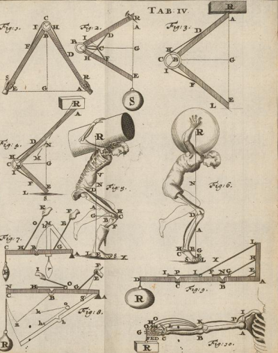
# # Figures from De motu animalium by Giovanni Alfonso Borelli (1608-1679), the father of biomechanics, depicting a static analysis of forces acting on the human body. #

# # In the mechanical modelling of an inanimate or living system, composed by one or more bodies (bodies as units that are mechanically isolated according to the question one is trying to answer), it is convenient to isolate each body (be they originally interconnected or not) and identify each force and moment of force (torque) that act on this body in order to apply the laws of mechanics. # # **The free body diagram (FBD) of a mechanical system or model is the representation in a diagram of all forces and moments of force acting on each body, isolated from the rest of the system.** # # The term free means that each body, which maybe was part of a connected system, is represented as isolated (free) and any existent contact force is represented in the diagram as forces (action and reaction) acting on the formely connected bodies. Then, the laws of mechanics are applied on each body, and the unknown movement, force or moment of force can be found if the system of equations is determined (the number of unknown variables can not be greater than the number of equations for each body). # # How exactly a FBD is drawn for a mechanical model of something is dependent on what one is trying to find. For example, the air resistance might be neglected or not when modelling the movement of an object and the number of parts the system is divided is dependent on what is needed to know about the model. # # The use of FBD is very common in biomechanics; a typical use is to use the FBD in order to determine the forces and torques on the ankle, knee, and hip joints of the lower limb (foot, leg, and thigh) during locomotion, and the FBD can be applied to any problem where the laws of mechanics are needed to solve a problem. # ## Equilibrium conditions # # In a static situation, the following equilibrium conditions, derived from Newton-Euler's equations for linear and rotational motions must be satisfied for each body under analysis using FBD: # # $$ \begin{array}{l l} # \sum \mathbf{F} = 0 \\ # \\ # \sum \mathbf{M} = 0 # \end{array} $$ # # That is, the **vectorial** sum of all forces and moments of force acting on the body must be zero hence the body is not moving or rotating. # And this must hold in all directions if we use the Cartesian coordinate system because the movement is independent in the orthogonal directions: # # $$ \sum \mathbf{F} = 0 \;\;\;\implies\;\;\; # \begin{array}{l l} # \sum F_x = 0 \\ # \sum F_y = 0 \\ # \sum F_z = 0 # \end{array} $$ # # $$ \sum \mathbf{M} = 0 \;\;\implies\;\;\; # \begin{array}{l l} # \sum M_x = 0 \\ # \sum M_y = 0 \\ # \sum M_z = 0 # \end{array} $$ # # 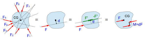Although many forces and moments of force can actuate on a rigid body, their effects in terms of motion, translation and rotation of the body, are the same of a single force acting on the body center of gravity and a couple of antiparallel forces (or simply, a force couple) that generates a moment of force. This moment of force has the particularity that is not around a fixed axis of rotation and because of that it is also called free moment or pure moment. The next figure illustrates this principle: # #

# # Based on the concept of force couple, we can make a distinction between torque and moment of force: torque is the moment of force caused by a force couple. We can also refer to torque as the moment of a couple. This distinction is more common in Engineering Mechanics. # # The equilibrium conditions and the fact that a multiple force system can be reduced to a simpler system will be useful to guide the drawing of a FBD. # Other important principles for a mechanical analysis are the principle of moments and the principle of transmissibility: # # ### Varignon's Theorem (Principle of moments) # # > *The moment of a force about a point is equal to the sum of moments of the components of the force about the same point.* # Note that the components of the force don't need to be orthogonal. # # ### Principle of transmissibility # # > *For rigid bodies with no deformation, an external force can be applied at any point on its line of action without changing the resultant effect of the force.* # # **Example** (From Meriam 1997). For the figure below, calculate the magnitude of the moment about the base point *O* of the 600-N force in five different ways[.](http://ebm.ufabc.edu.br/wp-content/uploads/2013/02/torque.png) # #

# # One way: # In[1]: import numpy as np M = np.cross([2,4,0], [600*np.cos(40*np.pi/180), -600*np.sin(40*np.pi/180),0]) print("The magnitude of the moment of force is: %d Nm" %np.around(np.linalg.norm(M))) # Let's start using the FBD to solve simple problems in mechanics. # # ## Example 1: Ball resting on the ground # # Our interest is to draw the FBD for the ball: #
#

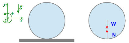
FBD01 — *Figure. Free-body diagram of a ball resting on the ground.*

# # W is the weight force due to the gravitational forces which act on all particles of the ball but the effects of the weight force on each particle of the ball are the same if we draw only one force (the ball weight) acting on the center of gravity of the ball. # N is the normal force, it is perpendicular to the surface of contact and prevents the ball from penetrating the surface. # # The vector representing a force must be drawn with its origin at the point of application of the force. However, for sake of clarity one might draw the contect forces outside the body with the tip of the vector at the contact region (note that in the figure above, we had to draw small vectors to avoid the superposition of them). # It is not necessary to draw the body in the FBD, just the vectors representing the forces would be enough. # # The ball also generates forces on the ground (the ball attracts the Earth with the same force but opposite direction and pushes the ground downwards), but since the question was to draw the FBD for the ball only, we don't need to care about that. # # When drawing a FBD, it's not necessary to portrait the body with details; one can draw a simple line to represent the body or nothing at all, only caring to draw the forces and moments of force in the right places. # # From the FBD, one can now derive the equilibrium equations: # In the vertical direction (there's nothing at the horizontal direction): # # $$ \mathbf{N}+\mathbf{W}=0 \;\;\; \implies \;\;\; \mathbf{N}=-\mathbf{W} $$ # # Where $\mathbf{W}=m\mathbf{g}\;\;(g=-10 m/s^2)$. # # This very simple case already illustrates a common problem when drawing a FBD and deriving the equations: # Is W negative or positive? Is $\mathbf{W}$ representing a vector quantity that we don't explicitly express knowledge about its direction or we will express its direction with a sign? Will we substitute the symbol $\mathbf{W}$ by $m\mathbf{g}$ or $-m\mathbf{g}$? And in any of these cases, is $g$ equals to $10$ or $-10 m/s^2$? # # This problem is known as double negative and it happens when we negate twice something we wanted to express as negative, for example, $\mathbf{W}=-m\mathbf{g}$, where $g=-10 m/s^2$. Be carefull and consistent with the convention adopted. # # If in the reference system we chose, the upward direction is positive, the value of $\mathbf{W}$ should be negative. # So, if we write the equation as $\mathbf{N}+\mathbf{W}=0$, it's because we are representing the vectors and the value of $\mathbf{W}$ is either equal to $m\mathbf{g}$ (with $g=-10 m/s^2$) or $-m\mathbf{g}$ (with $g=10 m/s^2$). # It would be also correct to write the equation as $\mathbf{N}-\mathbf{W}=0$ where $\mathbf{W}$ is equal to $m\mathbf{g}$ (with $g=10 m/s^2$), but the problem with this convention is that we are constraining the direction of the vector to only one possibility, but this might not be always true. # # The best option is to draw and write in the equations in vectorial form, without their signals and let the signals appear when the numerical values for these quantities are inputted. # But it is really a matter of convention, once a convention is adopted, you should grab it with all your forces! # ## Example 2: Person standing still # # Our interest is to draw the FBD for a person standing still: #
#

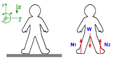
FBD02 — *Figure. Free-body diagram of a person standing.*

# # The FBD for the standing person above is similar to the previous one; the difference is that now there are two surfaces of contact (the two feet). And under each foot, there is an area of contact, not just a single point. # # In somewhat similar to the center of gravity, it is possible to compute a center of force, representing the point of application of the resultant vertical force of the ground on the foot (and it is even possible to compute a single center of force considering both feet). # # $\mathbf{N_1}$ and $\mathbf{N_2}$ are the normal forces acting on the feet and they were arbitrarily drawn acting on the middle of the foot, but the subject could stand in such a way that the center of force could be in the toes, for example. # # To exactly determine where the center of force is under each foot, we need an instrument to measure these forces and the point of application of the resultant vertical force. One instrument for that, used in biomechanics, is the force plate or force platform. In biomechanics, the center of force in this context is usually called center of pressure. # # Let's derive the equilibrium equation only for the forces in the vertical direction: # # $$ \mathbf{N_1}+\mathbf{N_2}+\mathbf{W}=0 \;\;\; \implies \;\;\; \mathbf{N_1}+\mathbf{N_2}=-\mathbf{W} $$ # # Where $\mathbf{W}=m\mathbf{g}\;\;(g=-10 m/s^2).$ # # This FBD, although simple, has already a complication to be solved: if the body is at rest, we know that the magnitude of the weight is equal to the magnitude of the sum of $\mathbf{N_1}$ and $\mathbf{N_2}$, but we are unable to determine $\mathbf{N_1}$ and $\mathbf{N_2}$ individually (the person could stand with more weight on one leg than in the other). But the total center of force between $\mathbf{N_1}$ and $\mathbf{N_2}$ must be exactly in the line of action of the weight force otherwise a moment of force will appear and the body will rotate. 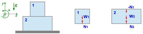# ## Example 3: Two boxes on the ground # # Our interest is to draw the FBD for both boxes: #
#

FBD03 — *Figure. Free-body diagram of two boxes on the ground.*

# # Now we have to consider the forces between the two boxes. # # Note that the forces $\mathbf{W_1}$ e $\mathbf{W_2}$ are the gravitational forces due to Earth. The boxes also attract each other but these forces are negligible and we don't need to draw them. # # The FBD for box 1 is the same as we drew for the ball before. For the box 2, as it acts on box 1 with the contact force $\mathbf{N_1}$ (the normal force) that prevents the box 1 from penetrating the surface of box 2, box 1 reacts with the same magnitude of force but in opposite direction, this is the force $\mathbf{-N_1}$. # # Remember from Newton's third law that the action and reaction force act on different bodies and these forces do not cancel each other. # # Let's derive the equilibrium equation only for the forces in the vertical direction: # # For body 1: # # $$ \mathbf{N_1}+\mathbf{W_1}=0 \;\;\; \implies \;\;\; \mathbf{N_1}=-\mathbf{W_1} $$ # # For body 2: # # $$ \mathbf{N_2}+\mathbf{W_2}-\mathbf{N_1}=0 \implies \;\;\; \mathbf{N_2}=-\mathbf{W_2}+\mathbf{N_1} \;\;\; \implies \;\;\; \mathbf{N_2}=-\mathbf{W_2}-\mathbf{W_1} $$ # # Where $\mathbf{W_1}=m_1\mathbf{g}\;\;\text{and}\;\;\mathbf{W_2}=m_2\mathbf{g}\;\;(g=-10 m/s^2).$ # # Note that the magnitude of $\mathbf{N_1}$ is equal to the magnitude of $\mathbf{W_1}$ and the magnitude of $\mathbf{N_2}$ is equal to the sum of the magnitudes of $\mathbf{W_1}$ and $\mathbf{W_2}$. # # At the end of the first example it's written: "The best option is to draw and write in the equations, the vectors, without their signals and let the signals appear when the numerical values for these quantities are inputted." # If this is to be followed, why then the representation of $-\mathbf{N_1}$ acting on body 2 in the FBD? # # The answer is that this is a different minus sign; it means that whatever is the value of this force, it should be the opposite of the normal force acting on body 1. 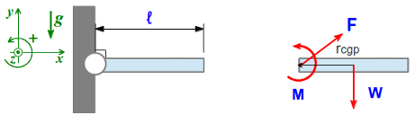# # ## Example 4: One segment fixed to a base (no movement) # # Now we have a segment fixed to a base by a joint and we want to draw the FBD for the segment: #
#

FBD04 — *Figure. Free-body diagram of one segment and one joint.*

# # On any joint one can have a force and a moment of force (but a joint with a free axis of rotation, offering no resistance to rotation, generates no moment of force, only joint forces). # For this example, we guessed the most general case, a joint with a force and a moment of force, but we may find later that one of these quantities is zero, this is ok. # And we arbitrarily chose the directions for joint force and moment of force; the actual directions don't matter now, but if we can choose any one, let's be positive! # # Forces: # # $$ # \mathbf{F} + \mathbf{W} = 0 \;\;\;\implies\;\;\; # \begin{array}{l l} # \mathbf{F_{x}} + 0 = 0 \;\;\;\implies\;\;\; \mathbf{F_{x}} = 0 \\ # \mathbf{F_{y}} + \mathbf{W} = 0 \;\;\;\implies\;\;\; \mathbf{F_{y}} = -\mathbf{W} \\ # \end{array} $$ # # Moments of force around the center of gravity of the segment: # # $$ \mathbf{M}+\mathbf{r_{cgp}}\times\mathbf{F}=0 \;\;\; \implies \;\;\; \mathbf{M}+\frac{\ell}{2}W=0 \;\;\; \implies \;\;\; \mathbf{M}=-\frac{\ell}{2}m\mathbf{g} $$ # # Remember that the direction of $\mathbf{M}$ is perpendicular to the plane of the FBD, it is in the $\mathbf{z}$ direction, because of the cross product. # # Where $\mathbf{r_{cgp}}$ is the position vector from the center of gravity to the proximal joint and $\mathbf{W}=m\mathbf{g}\;(g=-10 m/s^2)$. # # We can calculate the moment of force around any point that the condition of equilibrium must hold. In this example, we could have calculated the moment of force direct around the joint; in this case the weight causes a moment of force and the joint force does not. # # To find the direction of the moment of force might be difficult sometimes. If we had numbers for all these variables, we could simply do the mathematical operations and let the results indicate the direction. # For example, suppose the center of gravity is at the origin and that the bar has mass 1 kg and length 1 m. # Writing the equilibrium equation for the moments of force around the center of gravity, the moment of force at the joint is: # In[2]: m, l, g = 1.0, 1.0, -10.0 # m = 1kg, l = 1m, g = -10 m/s2 r = [-l/2-0, 0, 0] # note how the position vector from origin to F is created: tip minus tail F = [0, -m*g, 0] # this is the joint force not the gravitational force M = -np.cross( r, F ) print("The moment of force at the joint is (in Nm):", M) # The moment of force $\mathbf{M}$ is positive (counterclockwise direction) to balance the negative moment of force due to the gravitational force. # Note that $\mathbf{M}$ is a vector with three components, where only the third component, in the $\mathbf{z}$ direction, is nonzero (because $\mathbf{r}$ and $\mathbf{F}$ where both in the plane $\mathbf{xy}$). # # And writing the equilibrium equation for the moments of force around the joint, the moment of force at the joint is: # In[3]: m, l, g = 1.0, 1.0, -10.0 # m = 1kg, l = 1m, g = -10 m/s2 r = [l/2-0, 0, 0] # note how the position vector from origin to W is created: tip minus tail F = [0, m*g, 0] # this is the gravitational force M = -np.cross( r, F ) print("The moment of force at the joint is (in Nm):", M) # The same result, of course. 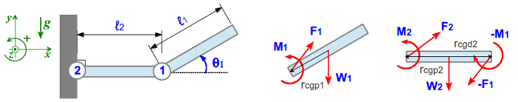# ## Example 5: Two segments and two joints # # Now we have two segments and two joints and we want to draw the FBD for each segment: #
#

FBD05 — *Figure. Free-body diagram of two segments and two joints.*

# # Note that the action-reaction principle applies to both forces and moments of force. # # In the FBD we draw the vectors representing forces and moments of forces without knowing their magnitude and direction. For example, the fact we drew the force F1 pointing upward and to the right direction is arbitrary. The calculation may reveal that this force points in fact to the opposite direction. There is no problem with that, the FBD is just an initial representation of all forces and moments of forces in the mechanical model. But once an arbitrary direction is chosen, we have to be consistent in representing the reaction forces and moments of forces. # # In a joint it may actuate more than one force and one moment of force. For example, for a human joint, typically there are many tendons and ligaments crossing the joint and the articulation has a region of contact. However, as we saw earlier, all the forces and moments of force can be reduced to a single force acting on the joint center (in fact to any point we desire) and to a free moment (a force couple) as we just drew. # # Let's derive the equilibrium equations for the forces and moments of force around the center of gravity: # # For body 1: # # $$ \mathbf{F_1} + \mathbf{W_1} = 0 $$ # # $$ \mathbf{M_1} + \mathbf{r_{cgp1}}\times\mathbf{F_1} = 0 $$ # # # For body 2: # # $$ \mathbf{F_2} + \mathbf{W_2} - \mathbf{F_1} = 0 $$ # # $$\mathbf{M_2} + \mathbf{r_{cgp2}}\times\mathbf{F_2} + \mathbf{r_{cgd2}}\times-\mathbf{F_{2}} - \mathbf{M_1} = 0 $$ # # Where **p** and **d** stands for proximal and distal joints (with respect to the fixed extremity) and $\mathbf{r_{cg\:ji}}$ is the position vector from the center of gravity of body **i** to the joint **j**. # # It is not possible to solve the problem starting with the body 2 because for this body there are more unknown variables than equations (both joint forces and moments of force are unknown for body 2). If we start by body 1, there is only one unknown joint force and moment of force and the system is solvable. # # In general, this is the approach we should take in biomechanics: for a multi-body system, start with the body with least unknown variables which usually has a free extremity or it has a sensor in this extremity able to measure the unknown quantity. # # For body 1: # # Forces: # # $$ \mathbf{F_{1x}} + 0 = 0 \;\;\;\implies\;\;\; $$ # # $$\mathbf{F_{1x}} = 0 $$ # # $$\mathbf{F_{1y}} + \mathbf{W_1} = 0 \;\;\;\implies\;\;\; $$ # # $$\mathbf{F_{1y}} = -m_1\mathbf{g} $$ # # Moments of force (around $cg_1$): # # $$ \mathbf{M_1}+\frac{\ell_1}{2}cos(\theta_1)\mathbf{W_1}=0 \;\;\;\implies\;\;\; $$ # # $$ \mathbf{M_1}=-\frac{\ell_1}{2}cos(\theta_1)m_1\mathbf{g} $$ # # Where $\theta_1$ is the angle of segment 1 with the horizontal and $g=-10 m/s^2.$ # # For body 2: # # Forces: # # $$ \mathbf{F_{2x}} + 0 - \mathbf{F_{1x}} = 0 \;\;\;\implies\;\;\; $$ # # $$ \mathbf{F_{2x}} = 0 $$ # # $$ \mathbf{F_{2y}} + \mathbf{W_2} - \mathbf{F_{1y}} = 0 \;\;\;\implies\;\;\; $$ # # $$ \mathbf{F_{2y}} = -m_1\mathbf{g} - m_2\mathbf{g} $$ # # Moments of force (around $cg_2$): # # $$ \mathbf{M_2} - \frac{\ell_2}{2}\mathbf{F_{2y}} - \frac{\ell_2}{2}\mathbf{F_{1y}} - \mathbf{M_1} = 0 \;\;\;\implies\;\;\; $$ # # $$ \mathbf{M_2} + \frac{\ell_2}{2}(m_1\mathbf{g} + m_2\mathbf{g}) + \frac{\ell_2}{2}m_1\mathbf{g} + \frac{\ell_1}{2}cos(\theta_1)m_1\mathbf{g} = 0 \;\;\;\implies\;\;\; $$ # # $$ \mathbf{M_2} = -\frac{\ell_2}{2}m_2\mathbf{g} - \left(\ell_2 + \frac{\ell_1}{2}cos(\theta_1)\right)m_1\mathbf{g} $$ # # Where $g=-10 m/s^2.$ # # This solution makes sense: # # - The force in joint 1 is the necessary force to support the weight of body 1, while the force in joint 2 is the necessary force to support the weight of bodies 1 and 2. # - Both $\mathbf{M_1}$ and $\mathbf{M_2}$ should be positive (counterclockwise direction) because these joint moments of force are necessary to support the bodies against gravity (which generates a negative (clockwise direction) moment of force on the joints). # - The magnitudes of the moments of force due to the weight of each body are simply the product between the correspondent body weight and the horizontal distance of the body center of gravity to the joint. # # This problem could have been solved calculating the moments of force around each joint instead of around the center of gravity; maybe it would have been simpler, but it would give the same results. # You are invited to check that. # ## The case of an accelerated rigid body # # The formalism above can be extended for an accelerated rigid body where the following conditions must be satisfied: # # $$ \sum \mathbf{F} = m\mathbf{a_{cm}} $$ # # $$ \sum \mathbf{M_O} = \frac{d\mathbf{L_O}}{dt} $$ # # Where $O$ is a reference point from which the movement (translation and rotation) of the rigid body is described ($O$ is an arbitrary position, it can be in any place in space). # The equations above are called dynamic equations. # # For a two-dimensional movement and if the reference point $O$ is at the body center of mass (i.e., for a rotation around the center of mass), the dynamic equations become: # # $$ \sum F_x = ma_{cm,x} $$ # # $$ \sum F_y = ma_{cm,y} $$ # # $$ \sum M_z = I_{cm}\alpha_z $$ # # Where $\mathbf{z}$ is the axis of rotation passing through the body center of mass and perpendicular to the plane of movement. # # If the reference point $O$ does not coincide with the body center of mass, the sum of moments of force on this point, $\sum M_{z,O}$, is equal to the sum of moments of force around the center of mass, $\sum M_{z,cm}$, plus the moment of force due to the sum of the external forces, $\sum\mathbf{F}=m\mathbf{a}_{cm}$, acting on the center of mass in relation to point $O$: # # $$ \sum M_{z,O} = I_{cm}\alpha_z + \mathbf{r}_{cm,O}\times m \mathbf{a}_{cm} $$ # # The equation above can also be understood as: the time rate of change of the total angular momentum around a reference point $O$, $d\mathbf{L_O}/dt$, is equal to the time rate of change of the angular momentum around the body center of mass, $I_{cm}\alpha_z$, plus the time rate of change of the angular momentum of the body center of mass around the reference point $O$, $\mathbf{r}_{cm,O}\times m \mathbf{a}_{cm}$. # # In a variation of the equation above, the vector product at the right side can be solved if we compute $d$, the (perpendicular) distance to the line of action of the acceleration vector: # # $$ \sum M_{z,O} = I_{cm}\alpha_z + m \mathbf{a}_{cm}d $$ # # Note that if the linear acceleration vector $\mathbf{a}_{cm}$ passes through the reference point $O$, $d=0$, and the equation above becomes the equation for a rotation around the center of mass. # We can express the moment of inertia around the reference point $O$ instead of around the body center of mass, in this case, the linear acceleration will also be expressed as the acceleration of the reference point $O$: # # $$ \sum M_{z,O} = I_{O}\alpha_z + \mathbf{r}_{cm,O}\times m \mathbf{a}_O $$ # # If the acceleration vector $\mathbf{a}_O$ passes through the center of mass, the cross product is zero and the equation above reduces to a simpler case (but now not around the body center of mass). And there is another condition where a simplification also occurs: if the acceleration $\mathbf{a}_O$ is zero, that is, if the reference point $O$ is fixed, the cross product is zero again. # # Which reference point to use for solving the dynamic equations is usually a matter of what turns the solution simpler. For example, if the rotation of the body occurs around a fixed axis, it is convenient to sum the momentts of force around this axis to eliminate the unknown force in the axis. In human motion analysis, particularly in the three-dimensional case, summing the moments of force around the body center of mass is typically simpler. # ## Example 6: example 5 with one segment accelerated # # Consider that the segment 1 of example 5 is accelerated with linear acceleration $\mathbf{a}_1$, angular acceleration $\alpha_1$, has a moment of inertia around its center of gravity $I_1$, and this movement happens in the plane (so, the vector $\alpha_1$ is has the $\mathbf{z}$ direction). # # Now, the dynamic equations for the forces and moments of force around the center of gravity are: # # For body 1: # # $$ \mathbf{F_1} + \mathbf{W_1} = m_1a_1 $$ # # $$ \mathbf{M_1} + \mathbf{r_{cgp1}}\times\mathbf{F_1} = I_1\alpha_1 $$ # # So, for the forces: # # $$ \mathbf{F_{1x}} + 0 = m_1a_{1x} \;\;\;\implies\;\;\; $$ # # $$\mathbf{F_{1x}} = m_1a_{1x} $$ # # $$\mathbf{F_{1y}} + \mathbf{W_1} = m_1a_{1y} \;\;\;\implies\;\;\; $$ # # $$\mathbf{F_{1y}} = m_1a_{1y} - m_1\mathbf{g} $$ # # And for the moments of force (around $cg_1$): # # $$ \mathbf{M_1} + \frac{\ell_1}{2} sin(\theta_1)m_1a_{1x} - \frac{\ell_1}{2} cos(\theta_1)(m_1a_{1y} - m_1\mathbf{g}) = I_1\alpha_1 \;\;\;\implies\;\;\; $$ # # $$ \mathbf{M_1} = I_1\alpha_1 + \frac{\ell_1}{2} \left( cos(\theta_1)(m_1a_{1y} - m_1\mathbf{g}) - sin(\theta_1)m_1a_{1x} \right) $$ # # Where $g = -10 m/s^2$. # # The equations for segment 2 are the same as in example 5, as the values of $\mathbf{F_1}$ and $\mathbf{M_1}$ are different now because of the acceleration, so it will be the values of $\mathbf{F_2}$ and $\mathbf{M_2}$. # # We also can solve the dynamic equation for the moments of force, now around the joint 1: # # $$ \mathbf{M_1} + \mathbf{r_{cgp1}}\times\mathbf{W_1} = I_1\alpha_1 + \mathbf{r}_{1cm,j1}\times m \mathbf{a}_1 \;\;\;\implies\;\;\; $$ # # $$ \mathbf{M_1} + \frac{\ell_1}{2}cos(\theta_1)m_1\mathbf{g} = I_1\alpha_1 - \frac{\ell_1}{2}sin(\theta_1)m_{1}a_{1x} + \frac{\ell_1}{2}cos(\theta_1)m_{1}a_{1y} \;\;\;\implies\;\;\; $$ # # $$ \mathbf{M_1} = I_1\alpha_1 + \frac{\ell_1}{2} \left( cos(\theta_1)(m_{1}a_{1y} - m_1\mathbf{g}) - sin(\theta_1)m_{1}a_{1x} \right) $$ # # Same result as before, of course. # ## Problems # # 1. Estimate the moments of force exerted by a $1kg$ ball to be held by you with outstretched arm horizontally relative to an axis that passes through: # a) Pulse # b) Elbow # c) Shoulder # # 2. A person performs isometric knee extension using a boot of $200N$ weight. Consider that the distance between the boot center of gravity and the center of the knee is $0.40 m$; that the quadriceps tendon is inserted at $5 cm$ from the joint in a 30$^o$ angle, that the mass of the leg + foot is $4 kg$, that the center of gravity of the leg + foot is $20 cm$ from the center of the knee joint, and that at a $0^o$ the knee is extended. # a) Calculate the muscle and joint forces at the knee angles 0$^o$, 45$^o$, and 90$^o$. 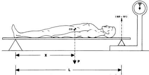# # 3. A simple and clever device to estimate the position of the center of mass position on a body is the reaction board illustrated below. #

Reaction board — *Figure. Illustration of the reaction board device for the estimation of the center of mass position on a body.*

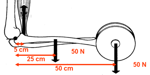
# # a) Derive the equation to determine the center of mass position considering the parameters shown in the figure above. # b) Show that it's possible to estimate the mass and center of mass position of a segment by asking the subject to move his or her segment and recalculating the center of mass position. # # 4. Consider the situation illustrated in the figure below where a person is holding a dumbbell. #

lever arm — *Figure. A person holding a dumbbell and some of the physical quantities related to the mechanics of the task.*

# # a) Determine the value of the elbow flexion force. # b) Determine the forces acting on the elbow joint. # # 5. What are the average moment of force (torque) and force that must be applied by the shoulder flexor muscle for a period of 0.3 s to stop the motion of the upper limb with angular speed of $5 rad/s$? Consider a radius of giration for the upper limb of $20 cm$; a mass of the upper limb of $3.5 kg$, and that the shoulder flexor muscle is inserted at a distance of $1.5 cm$ from the shoulder perpendicular to the axis of rotation. # # 6. Consider the system in Example 4, but now the segment (with $1m$ length and $4kg$ mass) is attached to the base by a joint that allows free rotation around the $\mathbf{z}$ axis. At the instant shown in Example 4 (at the horizontal), the segment has an angular velocity equals to $-5 rad/s$. Consider $g=-10 m/s^2$. 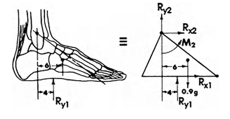For this instant, determine: # a) The angular acceleration # b) The force at the joint # c) The moment of force at the joint # # 7. Consider the foot segment during standing still (foot acceleration is zero) where the entire body is supported by the foot as illustrated in the figure. The distance in relation to the ankle joint of the foot center of mass is $6 cm$ and of the point of application of the resultant ground reaction force (center of pressure, COP) is $4 cm$ as illustrated in the figure. The foot mass is $0.9 kg$ and the ground reaction force (Ry1) is $588 N$. Consider $g=-9.8 m/s^2$. #

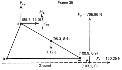
# # a) Determine the moment of force and force at the ankle. # # 8. Consider the foot segment at an instant during gait when the entire body is supported by the foot as illustrated in the figure. The coordinates of the ankle joint, foot center of mass and the point of application of the resultant ground reaction force (center of pressure, COP) are given in centimeters at the laboratory coordinate system. The foot accelerations are $a = (3.25, 1.78) m/s^2$, and $\alpha_z = −45.35 rad/s^2$ and the moment of inertia is $0.01 kgm^2$. Consider $g=-9.8 m/s^2$. #

# # a) Determine the moment of force and force at the ankle. # # 9. Study the content and solve the exercises of the text [Forces and Torques in Muscles and Joints](http://cnx.org/contents/d703853c-6382-4035-8d6a-dcbca00a15ca/Forces_and_Torques_in_Muscles_). # ## References # # - Hibbeler RC (2012) [Engineering Mechanics: Statics](http://books.google.com.br/books?id=PSEvAAAAQBAJ). Prentice Hall; 13 edition. # - Hibbeler RC (2012) [Engineering Mechanics: Dynamics](http://books.google.com.br/books?id=mTIrAAAAQBAJ). Prentice Hall; 13 edition. # - Ruina A, Rudra P (2013) [Introduction to Statics and Dynamics](http://ruina.tam.cornell.edu/Book/index.html). Oxford University Press. # - Winter DA (2009) [Biomechanics and motor control of human movement](http://books.google.com.br/books?id=_bFHL08IWfwC). 4 ed. Hoboken, EUA: Wiley. # - Zatsiorsky VM (2002) [Kinetics of human motion](http://books.google.com.br/books?id=wp3zt7oF8a0C). Champaign, IL: Human Kinetics.