#!/usr/bin/env python
# coding: utf-8
# # "Implement Markowitz Portfolio Optimization in Only 3 Lines of Code"
# > "Use fastquant to maximize the returns of your stock portfolio given its overall risk profile"
#
# - toc: true
# - branch: master
# - badges: true
# - comments: true
# - author: Benjamin Cabalona, Jerome de Leon
# - categories: [portfolio, optimization]
# In[1]:
# uncomment to install in colab
# !pip3 install fastquant
#  # # Some Basic Ideas
#
# **Stock or Share** is a unit of ownership in a company. When you invest in the stock market, (stock market is basically a place for buying or selling stocks) there are 2 main ways of earning:
#
# - **Dividend** - This is an amount paid to you by a company for your investment.
# - **Stock Trading** - The profit that you make for buying/selling stocks.
# - **Portfolio** - A combination of assets of an individual / investor.
#
# Fundamentally, you can earn money by buying some stocks, in the hope that it's price will increase in the future.
#
# There are actually clever ways on how to earn even if you predict that a stock price will decline, but that's outside the scope of this lecture.
#
# So in this lecture, we'll oversimplify and what we want is to **buy a stock cheap, and sell it when its price has increased** because that way we will make a profit. Otherwise we will incur a loss, if we decided to sell a stock at a cheaper price.
#
# # Modern Portfolio Theory (Markowitz Model)
#
# As mentioned above, investing in the stock market can result in either profit or loss.
#
# In a nutshell, Modern Portfolio Theory is a way of maximizing return for a given risk. We will define what *return* and *risk* means shortly.
#
# Let's understand this by using an example.
#
# Suppose you wanted to invest in the stock market. After completing your research, you decided to invest in the following companies:
#
# - MEG
# - MAXS
# - JFC
# - ALI
#
# We will download the data for this using a python library called fastquant. It was actually developed by a fellow Filipino Data Scientist. It aims to democratize data-driven investments for everyone.
#
#
# **NOTE** The model we'll be using relies on the assumption that returns are normally distributed. Therefore, it helps if we have large number of data points.
# In[2]:
import pandas as pd
import numpy as np
import matplotlib.pyplot as plt
import warnings
import scipy.optimize as optimization
from fastquant import get_stock_data
warnings.filterwarnings('ignore')
get_ipython().run_line_magic('matplotlib', 'inline')
# In[3]:
stocks = ['MEG', 'MAXS', 'JFC', 'ALI']
datas = []
for i in stocks:
df = get_stock_data(i, "2017-01-01", "2020-01-01")
df = df.reset_index()
df.columns = ['DATE',i]
df = df[['DATE',i]]
datas.append(df)
datas1 = pd.merge(datas[0],datas[1],on=['DATE'])
datas2 = pd.merge(datas[2],datas[3],on=['DATE'])
data = pd.merge(datas1,datas2,on=['DATE'])
data.index = data['DATE']
data.drop('DATE',axis=1,inplace=True)
# The table below shows the first 5 entries in our dataset. The values here are *closing prices*. A *closing price* is a price of a stock at the end of a given trading day.
# In[4]:
data.head()
# Now, let's ask ourselves. Why don't we invest in a single company, instead of investing in multiple companies?
#
# Modern Portfolio Theory tells us that we can *minimize* our loss thru diversification. Let's understand this with an example.
#
# Suppose you decided to invest on January 2017. For illustraton purposes, let's consider the period January 2017 - May 2018.
#
# - Case 1: You invested solely on MAXS
# - Case 2: You decided to invest 50% to MAXS and the other 50% to JFC
#
# If you decided to go with case 1, it would be clear that you could immediately lose some money (as the chart shows a decreasing trend). If you instead decided to go with Case 2, your loss could have been mitigated since the price for JFC is increasing during that period.
#
# Of course you could argue that "why not invest all of my money in JFC", well my counter argument to that would be, when JFC is experiencing a decline in it's price, there would be some other company that's actually experiencing an increase in it's price.
#
# ## Key Takeaway
#
# - Invest in multiple stocks as much as possible, to minimize your loss. (Technically uncorrelated or negatively correlated)
# In[5]:
data['MAXS'].plot(figsize=(12,5),legend=True)
# In[6]:
data['JFC'].plot(figsize=(12,5),legend=True,color='r')
# Now, let's define what a return is. Intuitively, we can define return as :
#
# *The stock price today minus the stock price yesterday. Divide the difference by the stock price yesterday*
#
# More formally,
#
# The *return* $R_{t,t+1}$ from time $t$ to time ${t+1}$ is given by:
#
# $$ R_{t,t+1} = \frac{P_{t+1}-P_{t}}{P_{t}} $$
#
# where $P_i$ is the price of the stock for a given time point.
# In[7]:
returns = data.pct_change()
returns
# The mean of the returns is called the **Expected Return**.
#
# Similarly, the **Risk or Volatility** is the standard deviation of the returns.
#
# (This is different from the expected return and volatility of a portfolio, this is for a single stock)
# In[8]:
returns.mean()
# In[9]:
returns.std()
# We'll only plot MAXS and MEG to emphasize that the return for MEG is more volatile.
# In[10]:
returns[['MAXS','MEG']].plot(figsize=(12,5))
# ## Expected Return and Risk of a Portfolio
#
# Suppose your portfolio consists of returns $R_1, R_2, R_3, ... ,R_n$. Then, the expected return of a portfolio is given by:
#
# $E(R) = w_1E(R_1) + w_2E(R_2) + w_3E(R_3) + ... + w_nE(R_n) $
#
# where $w_i$ is the $i$th component of an $n-dimensional$ vector, and $\Sigma w_i = 1.$
# In[11]:
weights = np.random.random(len(stocks))
weights /= np.sum(weights)
weights
# In[12]:
returns.mean()
# In[13]:
def calculate_portfolio_return(returns, weights):
portfolio_return = np.sum(returns.mean()*weights)*252
print("Expected Portfolio Return:", portfolio_return)
# In[14]:
calculate_portfolio_return(returns,weights)
# If you had a course in Probability, you might recall that expectation of a random variable is linear while the variance is not. That's the same argument why the formula for the variance of a portfolio is quite more complicated.
#
# $Var(R) = \bf{w^{T}}\Sigma \textbf{w}$
#
# where $\Sigma$ is the covariance matrix of $R_i$
# In[15]:
returns.cov()
# In[16]:
np.sqrt(returns.cov())
# In[17]:
returns.std()
# In[18]:
def calculate_portfolio_risk(returns, weights):
portfolio_variance = np.sqrt(np.dot(weights.T, np.dot(returns.cov()*252,weights)))
print("Expected Risk:", portfolio_variance)
# In[19]:
calculate_portfolio_risk(returns,weights)
# ## Sharpe Ratio
#
#
# Remember, what we want is to find the best possible weight vector $\bf{w}$ that would give us the best possible return, with a minimal risk. Therefore, we will introduce a new metric called the *sharpe ratio*. It's simply equal to
#
# $$S.R. = \frac{E(R) - R_f}{\sqrt{Var(R)}}$$
#
# where $R_f$ is the *risk free return*. Since we're only limiting ourselves to risky assets (stocks) therefore, the formula becomes
#
# $$S.R. = \frac{E(R) - 0}{\sqrt{Var(R)}} = \frac{E(R)}{\sqrt{Var(R)}}$$
# In[20]:
def generate_portfolios(weights, returns):
preturns = []
pvariances = []
for i in range(10000):
weights = np.random.random(len(stocks))
weights/=np.sum(weights)
preturns.append(np.sum(returns.mean()*weights)*252)
pvariances.append(np.sqrt(np.dot(weights.T,np.dot(returns.cov()*252,weights))))
preturns = np.array(preturns)
pvariances = np.array(pvariances)
return preturns,pvariances
def plot_portfolios(returns, variances):
plt.figure(figsize=(10,6))
plt.scatter(variances,returns,c=returns/variances,marker='o')
plt.grid(True)
plt.xlabel('Expected Volatility')
plt.ylabel('Expected Return')
plt.colorbar(label='Sharpe Ratio')
plt.show()
# In[21]:
preturns, pvariances = generate_portfolios(weights,returns)
# ## Monte - Carlo Simulation
#
# Here, we simulated 10,000 possible weight allocations, and computed their respective expected return, risk and sharpe ratio.
# In[22]:
plot_portfolios(preturns, pvariances)
# # Finding and plotting the Optimal Weights (the hard way)
#
# At a high level, we would want to run an optimization algorithm that would
#
#
# $$maximize\ \frac{E(R)-R_f}{\sqrt{Var(R)}}$$
#
# $$s.t. \forall w_i, w_i\geq0\ and\ \Sigma w_i=1$$
#
# Full details of the mathematics behind this can be found on resources.
# In[23]:
def statistics(weights, returns):
portfolio_return=np.sum(returns.mean()*weights)*252
portfolio_volatility=np.sqrt(np.dot(weights.T,np.dot(returns.cov()*252,weights)))
return np.array([portfolio_return,portfolio_volatility,portfolio_return/portfolio_volatility])
def min_func_sharpe(weights,returns):
return -statistics(weights,returns)[2]
def optimize_portfolio(weights,returns):
constraints = ({'type':'eq','fun': lambda x: np.sum(x)-1})
bounds = tuple((0,1) for x in range(len(stocks)))
optimum=optimization.minimize(fun=min_func_sharpe,x0=weights,args=returns,method='SLSQP',bounds=bounds,constraints=constraints)
return optimum
def print_optimal_portfolio(optimum, returns):
print("Optimal weights:", optimum['x'].round(3))
print("Expected return, volatility and Sharpe ratio:", statistics(optimum['x'].round(3),returns))
def show_optimal_portfolio(optimum, returns, preturns, pvariances):
plt.figure(figsize=(10,6))
plt.scatter(pvariances,preturns,c=preturns/pvariances,marker='o')
plt.grid(True)
plt.xlabel('Expected Volatility')
plt.ylabel('Expected Return')
plt.colorbar(label='Sharpe Ratio')
plt.plot(statistics(optimum['x'],returns)[1],statistics(optimum['x'],returns)[0],'g*',markersize=20.0)
plt.show()
# In[24]:
optimum=optimize_portfolio(weights,returns)
print_optimal_portfolio(optimum, returns)
show_optimal_portfolio(optimum, returns, preturns, pvariances)
# # Finding and plotting the Optimal Weights (the fastquant way)
#
# Since our goal is to promote data driven investments by making quantitative analysis in finance accessible to everyone, the markowitz model is also implemented in fastquant. All it takes is a few lines of code as shown below.
# In[25]:
from fastquant import Portfolio
# In[26]:
stock_list = ['MEG', 'MAXS', 'JFC', 'ALI']
p = Portfolio(stock_list,"2017-01-01", "2020-01-01")
axs = p.data.plot(subplots=True, figsize=(15,10))
fig = p.plot_portfolio(N=1000)
# # Bonus Section : Interactive Charts
#
# This section is expected to **NOT** render in github, but does in fastpages.
#
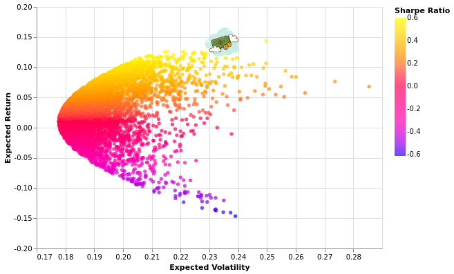
# It is expected to look like the image below, and in addition, the tooltip is interactive.
#
#
# # Some Basic Ideas
#
# **Stock or Share** is a unit of ownership in a company. When you invest in the stock market, (stock market is basically a place for buying or selling stocks) there are 2 main ways of earning:
#
# - **Dividend** - This is an amount paid to you by a company for your investment.
# - **Stock Trading** - The profit that you make for buying/selling stocks.
# - **Portfolio** - A combination of assets of an individual / investor.
#
# Fundamentally, you can earn money by buying some stocks, in the hope that it's price will increase in the future.
#
# There are actually clever ways on how to earn even if you predict that a stock price will decline, but that's outside the scope of this lecture.
#
# So in this lecture, we'll oversimplify and what we want is to **buy a stock cheap, and sell it when its price has increased** because that way we will make a profit. Otherwise we will incur a loss, if we decided to sell a stock at a cheaper price.
#
# # Modern Portfolio Theory (Markowitz Model)
#
# As mentioned above, investing in the stock market can result in either profit or loss.
#
# In a nutshell, Modern Portfolio Theory is a way of maximizing return for a given risk. We will define what *return* and *risk* means shortly.
#
# Let's understand this by using an example.
#
# Suppose you wanted to invest in the stock market. After completing your research, you decided to invest in the following companies:
#
# - MEG
# - MAXS
# - JFC
# - ALI
#
# We will download the data for this using a python library called fastquant. It was actually developed by a fellow Filipino Data Scientist. It aims to democratize data-driven investments for everyone.
#
#
# **NOTE** The model we'll be using relies on the assumption that returns are normally distributed. Therefore, it helps if we have large number of data points.
# In[2]:
import pandas as pd
import numpy as np
import matplotlib.pyplot as plt
import warnings
import scipy.optimize as optimization
from fastquant import get_stock_data
warnings.filterwarnings('ignore')
get_ipython().run_line_magic('matplotlib', 'inline')
# In[3]:
stocks = ['MEG', 'MAXS', 'JFC', 'ALI']
datas = []
for i in stocks:
df = get_stock_data(i, "2017-01-01", "2020-01-01")
df = df.reset_index()
df.columns = ['DATE',i]
df = df[['DATE',i]]
datas.append(df)
datas1 = pd.merge(datas[0],datas[1],on=['DATE'])
datas2 = pd.merge(datas[2],datas[3],on=['DATE'])
data = pd.merge(datas1,datas2,on=['DATE'])
data.index = data['DATE']
data.drop('DATE',axis=1,inplace=True)
# The table below shows the first 5 entries in our dataset. The values here are *closing prices*. A *closing price* is a price of a stock at the end of a given trading day.
# In[4]:
data.head()
# Now, let's ask ourselves. Why don't we invest in a single company, instead of investing in multiple companies?
#
# Modern Portfolio Theory tells us that we can *minimize* our loss thru diversification. Let's understand this with an example.
#
# Suppose you decided to invest on January 2017. For illustraton purposes, let's consider the period January 2017 - May 2018.
#
# - Case 1: You invested solely on MAXS
# - Case 2: You decided to invest 50% to MAXS and the other 50% to JFC
#
# If you decided to go with case 1, it would be clear that you could immediately lose some money (as the chart shows a decreasing trend). If you instead decided to go with Case 2, your loss could have been mitigated since the price for JFC is increasing during that period.
#
# Of course you could argue that "why not invest all of my money in JFC", well my counter argument to that would be, when JFC is experiencing a decline in it's price, there would be some other company that's actually experiencing an increase in it's price.
#
# ## Key Takeaway
#
# - Invest in multiple stocks as much as possible, to minimize your loss. (Technically uncorrelated or negatively correlated)
# In[5]:
data['MAXS'].plot(figsize=(12,5),legend=True)
# In[6]:
data['JFC'].plot(figsize=(12,5),legend=True,color='r')
# Now, let's define what a return is. Intuitively, we can define return as :
#
# *The stock price today minus the stock price yesterday. Divide the difference by the stock price yesterday*
#
# More formally,
#
# The *return* $R_{t,t+1}$ from time $t$ to time ${t+1}$ is given by:
#
# $$ R_{t,t+1} = \frac{P_{t+1}-P_{t}}{P_{t}} $$
#
# where $P_i$ is the price of the stock for a given time point.
# In[7]:
returns = data.pct_change()
returns
# The mean of the returns is called the **Expected Return**.
#
# Similarly, the **Risk or Volatility** is the standard deviation of the returns.
#
# (This is different from the expected return and volatility of a portfolio, this is for a single stock)
# In[8]:
returns.mean()
# In[9]:
returns.std()
# We'll only plot MAXS and MEG to emphasize that the return for MEG is more volatile.
# In[10]:
returns[['MAXS','MEG']].plot(figsize=(12,5))
# ## Expected Return and Risk of a Portfolio
#
# Suppose your portfolio consists of returns $R_1, R_2, R_3, ... ,R_n$. Then, the expected return of a portfolio is given by:
#
# $E(R) = w_1E(R_1) + w_2E(R_2) + w_3E(R_3) + ... + w_nE(R_n) $
#
# where $w_i$ is the $i$th component of an $n-dimensional$ vector, and $\Sigma w_i = 1.$
# In[11]:
weights = np.random.random(len(stocks))
weights /= np.sum(weights)
weights
# In[12]:
returns.mean()
# In[13]:
def calculate_portfolio_return(returns, weights):
portfolio_return = np.sum(returns.mean()*weights)*252
print("Expected Portfolio Return:", portfolio_return)
# In[14]:
calculate_portfolio_return(returns,weights)
# If you had a course in Probability, you might recall that expectation of a random variable is linear while the variance is not. That's the same argument why the formula for the variance of a portfolio is quite more complicated.
#
# $Var(R) = \bf{w^{T}}\Sigma \textbf{w}$
#
# where $\Sigma$ is the covariance matrix of $R_i$
# In[15]:
returns.cov()
# In[16]:
np.sqrt(returns.cov())
# In[17]:
returns.std()
# In[18]:
def calculate_portfolio_risk(returns, weights):
portfolio_variance = np.sqrt(np.dot(weights.T, np.dot(returns.cov()*252,weights)))
print("Expected Risk:", portfolio_variance)
# In[19]:
calculate_portfolio_risk(returns,weights)
# ## Sharpe Ratio
#
#
# Remember, what we want is to find the best possible weight vector $\bf{w}$ that would give us the best possible return, with a minimal risk. Therefore, we will introduce a new metric called the *sharpe ratio*. It's simply equal to
#
# $$S.R. = \frac{E(R) - R_f}{\sqrt{Var(R)}}$$
#
# where $R_f$ is the *risk free return*. Since we're only limiting ourselves to risky assets (stocks) therefore, the formula becomes
#
# $$S.R. = \frac{E(R) - 0}{\sqrt{Var(R)}} = \frac{E(R)}{\sqrt{Var(R)}}$$
# In[20]:
def generate_portfolios(weights, returns):
preturns = []
pvariances = []
for i in range(10000):
weights = np.random.random(len(stocks))
weights/=np.sum(weights)
preturns.append(np.sum(returns.mean()*weights)*252)
pvariances.append(np.sqrt(np.dot(weights.T,np.dot(returns.cov()*252,weights))))
preturns = np.array(preturns)
pvariances = np.array(pvariances)
return preturns,pvariances
def plot_portfolios(returns, variances):
plt.figure(figsize=(10,6))
plt.scatter(variances,returns,c=returns/variances,marker='o')
plt.grid(True)
plt.xlabel('Expected Volatility')
plt.ylabel('Expected Return')
plt.colorbar(label='Sharpe Ratio')
plt.show()
# In[21]:
preturns, pvariances = generate_portfolios(weights,returns)
# ## Monte - Carlo Simulation
#
# Here, we simulated 10,000 possible weight allocations, and computed their respective expected return, risk and sharpe ratio.
# In[22]:
plot_portfolios(preturns, pvariances)
# # Finding and plotting the Optimal Weights (the hard way)
#
# At a high level, we would want to run an optimization algorithm that would
#
#
# $$maximize\ \frac{E(R)-R_f}{\sqrt{Var(R)}}$$
#
# $$s.t. \forall w_i, w_i\geq0\ and\ \Sigma w_i=1$$
#
# Full details of the mathematics behind this can be found on resources.
# In[23]:
def statistics(weights, returns):
portfolio_return=np.sum(returns.mean()*weights)*252
portfolio_volatility=np.sqrt(np.dot(weights.T,np.dot(returns.cov()*252,weights)))
return np.array([portfolio_return,portfolio_volatility,portfolio_return/portfolio_volatility])
def min_func_sharpe(weights,returns):
return -statistics(weights,returns)[2]
def optimize_portfolio(weights,returns):
constraints = ({'type':'eq','fun': lambda x: np.sum(x)-1})
bounds = tuple((0,1) for x in range(len(stocks)))
optimum=optimization.minimize(fun=min_func_sharpe,x0=weights,args=returns,method='SLSQP',bounds=bounds,constraints=constraints)
return optimum
def print_optimal_portfolio(optimum, returns):
print("Optimal weights:", optimum['x'].round(3))
print("Expected return, volatility and Sharpe ratio:", statistics(optimum['x'].round(3),returns))
def show_optimal_portfolio(optimum, returns, preturns, pvariances):
plt.figure(figsize=(10,6))
plt.scatter(pvariances,preturns,c=preturns/pvariances,marker='o')
plt.grid(True)
plt.xlabel('Expected Volatility')
plt.ylabel('Expected Return')
plt.colorbar(label='Sharpe Ratio')
plt.plot(statistics(optimum['x'],returns)[1],statistics(optimum['x'],returns)[0],'g*',markersize=20.0)
plt.show()
# In[24]:
optimum=optimize_portfolio(weights,returns)
print_optimal_portfolio(optimum, returns)
show_optimal_portfolio(optimum, returns, preturns, pvariances)
# # Finding and plotting the Optimal Weights (the fastquant way)
#
# Since our goal is to promote data driven investments by making quantitative analysis in finance accessible to everyone, the markowitz model is also implemented in fastquant. All it takes is a few lines of code as shown below.
# In[25]:
from fastquant import Portfolio
# In[26]:
stock_list = ['MEG', 'MAXS', 'JFC', 'ALI']
p = Portfolio(stock_list,"2017-01-01", "2020-01-01")
axs = p.data.plot(subplots=True, figsize=(15,10))
fig = p.plot_portfolio(N=1000)
# # Bonus Section : Interactive Charts
#
# This section is expected to **NOT** render in github, but does in fastpages.
#
# It is expected to look like the image below, and in addition, the tooltip is interactive.
#
#  #
# Refer to this link https://altair-viz.github.io/getting_started/installation.html for altair's installation, but most likely
#
# ```python
# !pip3 install altair
# ```
#
# should do the trick.
# In[27]:
import altair as alt
alt.renderers.set_embed_options(actions=False)
# In[28]:
weights = pd.DataFrame(optimum['x'].round(2),columns=['weights'])
weights['Symbols'] = stocks
# In[29]:
returns,variances = p.generate_portfolios(N=5000)
portfolios = pd.DataFrame()
portfolios['Expected Return'] = returns
portfolios['Expected Volatility'] = variances
portfolios['Sharpe Ratio'] = portfolios['Expected Return'] / portfolios['Expected Volatility']
minimumX = portfolios['Expected Volatility'].min()
maximumX = portfolios['Expected Volatility'].max()
minimumY = portfolios['Expected Return'].min()
maximumY = portfolios['Expected Return'].max()
optimum = p.calculate_statistics(p.optimum_weights)
optimal = pd.DataFrame()
optimal['Expected Return'] = [optimum[0]]
optimal['Expected Volatility'] = [optimum[1]]
optimal['Sharpe Ratio'] = [optimum[2]]
optimal['img'] = "https://img.icons8.com/clouds/100/000000/us-dollar--v1.png"
# In[30]:
# uncomment if N > 5000
# alt.data_transformers.enable('json')
# In[31]:
chart = alt.Chart(portfolios).mark_circle().encode(
x = alt.X('Expected Volatility',scale=alt.Scale(domain=[minimumX,maximumX])),
y = alt.X('Expected Return',scale=alt.Scale(domain=[minimumY,maximumY])),
color = alt.Color('Sharpe Ratio',scale=alt.Scale(range=['blue','yellow'])),
tooltip = ['Sharpe Ratio']
).properties(height=350,width=500)
optimal_chart = alt.Chart(optimal).mark_image(height=60,width=60).encode(
x = alt.X('Expected Volatility',scale=alt.Scale(domain=[minimumX,maximumX])),
y = alt.X('Expected Return',scale=alt.Scale(domain=[minimumY,maximumY])),
color = alt.Color('Sharpe Ratio',scale=alt.Scale(range=['blue','yellow'])),
tooltip = ['Sharpe Ratio'],
url = 'img'
).properties(height=350,width=500)
visualization = chart+optimal_chart
visualization
# Resources:
#
# - Financial Mathematics
# - https://www.springer.com/gp/book/9780857290816
# - General Investing
# - https://www.ig.com/en/learn-to-trade/ig-academy
#
# Refer to this link https://altair-viz.github.io/getting_started/installation.html for altair's installation, but most likely
#
# ```python
# !pip3 install altair
# ```
#
# should do the trick.
# In[27]:
import altair as alt
alt.renderers.set_embed_options(actions=False)
# In[28]:
weights = pd.DataFrame(optimum['x'].round(2),columns=['weights'])
weights['Symbols'] = stocks
# In[29]:
returns,variances = p.generate_portfolios(N=5000)
portfolios = pd.DataFrame()
portfolios['Expected Return'] = returns
portfolios['Expected Volatility'] = variances
portfolios['Sharpe Ratio'] = portfolios['Expected Return'] / portfolios['Expected Volatility']
minimumX = portfolios['Expected Volatility'].min()
maximumX = portfolios['Expected Volatility'].max()
minimumY = portfolios['Expected Return'].min()
maximumY = portfolios['Expected Return'].max()
optimum = p.calculate_statistics(p.optimum_weights)
optimal = pd.DataFrame()
optimal['Expected Return'] = [optimum[0]]
optimal['Expected Volatility'] = [optimum[1]]
optimal['Sharpe Ratio'] = [optimum[2]]
optimal['img'] = "https://img.icons8.com/clouds/100/000000/us-dollar--v1.png"
# In[30]:
# uncomment if N > 5000
# alt.data_transformers.enable('json')
# In[31]:
chart = alt.Chart(portfolios).mark_circle().encode(
x = alt.X('Expected Volatility',scale=alt.Scale(domain=[minimumX,maximumX])),
y = alt.X('Expected Return',scale=alt.Scale(domain=[minimumY,maximumY])),
color = alt.Color('Sharpe Ratio',scale=alt.Scale(range=['blue','yellow'])),
tooltip = ['Sharpe Ratio']
).properties(height=350,width=500)
optimal_chart = alt.Chart(optimal).mark_image(height=60,width=60).encode(
x = alt.X('Expected Volatility',scale=alt.Scale(domain=[minimumX,maximumX])),
y = alt.X('Expected Return',scale=alt.Scale(domain=[minimumY,maximumY])),
color = alt.Color('Sharpe Ratio',scale=alt.Scale(range=['blue','yellow'])),
tooltip = ['Sharpe Ratio'],
url = 'img'
).properties(height=350,width=500)
visualization = chart+optimal_chart
visualization
# Resources:
#
# - Financial Mathematics
# - https://www.springer.com/gp/book/9780857290816
# - General Investing
# - https://www.ig.com/en/learn-to-trade/ig-academy