#!/usr/bin/env python
# coding: utf-8

# # Hierarchical time series
# 
# [![Binder](https://mybinder.org/badge_logo.svg)](https://mybinder.org/v2/gh/etna-team/etna/master?filepath=examples/303-hierarchical_pipeline.ipynb)

# This notebook contains examples of modelling hierarchical time series.
# 
# **Table of contents**
# 
# * [Hierarchical time series](#chapter1)
# * [Preparing dataset](#chapter2)
#     * [Manually setting hierarchical structure](#chapter2_1)
#     * [Hierarchical structure detection](#chapter2_2)
# * [Reconciliation methods](#chapter3)
#     * [Bottom-up approach](#chapter3_1)
#     * [Top-down approach](#chapter3_2)
# * [Exogenous variables for hierarchical forecasts](#chapter4)

# In[1]:


import warnings

warnings.filterwarnings("ignore")


# In[2]:


import pandas as pd

from etna.metrics import SMAPE
from etna.models import LinearPerSegmentModel
from etna.pipeline import HierarchicalPipeline
from etna.pipeline import Pipeline
from etna.transforms import LagTransform
from etna.transforms import OneHotEncoderTransform

pd.options.display.max_columns = 100


# ## 1. Hierarchical time series <a class="anchor" id="chapter1"></a>

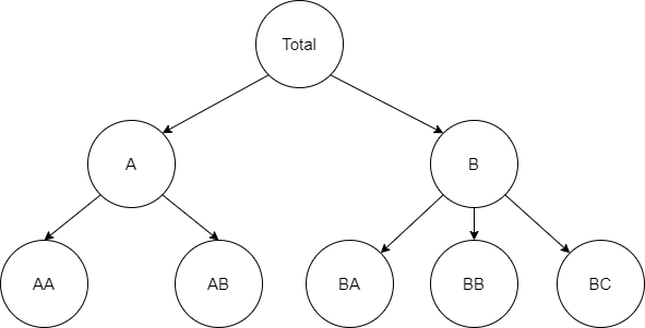
# In many applications time series have a natural level structure. Time series with such properties can be disaggregated by attributes
# from lower levels. On the other hand, this time series can be aggregated to higher levels to represent more general relations.
# The set of possible levels forms the hierarchy of time series.

# ![Hierarchy example](assets/hierarchical_pipeline/hierarchy.png)
# 
# *Two level hierarchical structure*

# Image above represents relations between members of the hierarchy. Middle and top levels can be disaggregated using members from
# lower levels. For example
# 
# $$
# y_{A,t} = y_{AA,t} + y_{AB,t}
# $$
# 
# $$
# y_{t} = y_{A,t} + y_{B,t}
# $$
# 

# In matrix notation level aggregation could be written as
# 
# $$
# \begin{equation}
#     \begin{bmatrix}
#         y_{A,t} \\
#         y_t
#     \end{bmatrix}
#     =
#     \begin{bmatrix}
#     1 & 1 & 0 \\
#     1 & 1 & 1
#     \end{bmatrix}
#     \begin{bmatrix}
#     y_{AA,t} \\ y_{AB,t} \\ y_{B,t}
#     \end{bmatrix}
#     =
#     S
#     \begin{bmatrix}
#     y_{AA,t} \\ y_{AB,t} \\ y_{B,t}
#     \end{bmatrix}
# \end{equation}
# $$
# 
# where $S$ - summing matrix.

# ## 2. Preparing dataset <a class="anchor" id="chapter2"></a>

# Consider the Australian tourism dataset.
# 
# This dataset consists of the following components:
# 
# * `Total` - total domestic tourism demand,
# * Tourism reasons components (`Hol` for holiday, `Bus` for business, etc)
# * Components representing the "region-reason" division (`NSW - hol`, `NSW - bus`, etc)
# * Components representing "region - reason - city" division (`NSW - hol - city`, `NSW - hol - noncity`, etc)
# 
# We can see that these components form a hierarchy with the following levels:
# 
# 1. Total
# 2. Tourism reason
# 3. Region
# 4. City

# In[3]:


get_ipython().system('curl "https://robjhyndman.com/data/hier1_with_names.csv" --ssl-no-revoke -o "hier1_with_names.csv"')


# In[4]:


df = pd.read_csv("hier1_with_names.csv")

periods = len(df)
df["timestamp"] = pd.date_range("2006-01-01", periods=periods, freq="MS")
df.set_index("timestamp", inplace=True)

df.head()


# ### 2.1 Manually setting hierarchical structure <a class="anchor" id="chapter2_1"></a>
# This section presents how to set hierarchical structure and prepare data. We are going to create a hierarchical
# dataset with two levels: total demand and demand per tourism reason.

# In[5]:


from etna.datasets import TSDataset


# Consider the **Reason** level of the hierarchy.

# In[6]:


reason_segments = ["Hol", "VFR", "Bus", "Oth"]

df[reason_segments].head()


# ### 2.1.1 Convert dataset to ETNA wide format <a class="anchor" id="chapter2_1_1"></a>
# First, convert dataframe to ETNA long format.

# In[7]:


hierarchical_df = []
for segment_name in reason_segments:
    segment = df[segment_name]

    segment_slice = pd.DataFrame(
        {"timestamp": segment.index, "target": segment.values, "segment": [segment_name] * periods}
    )
    hierarchical_df.append(segment_slice)

hierarchical_df = pd.concat(hierarchical_df, axis=0)

hierarchical_df.head()


# Now, the dataframe could be converted to ETNA wide format.

# In[8]:


hierarchical_df = TSDataset.to_dataset(df=hierarchical_df)


# ### 2.1.2 Creat HierarchicalStructure <a class="anchor" id="chapter2_1_2"></a>
# For handling information about hierarchical structure, there is a dedicated object in the ETNA library: `HierarchicalStructure`.
# 
# To create `HierarchicalStructure` define relationships between segments at different levels. This relation should be
# described as mapping between levels members, where keys are parent segments and values are lists of child segments
# from the lower level. Also provide a list of level names, where ordering corresponds to hierarchical relationships
# between levels.

# In[9]:


from etna.datasets import HierarchicalStructure


# In[10]:


hierarchical_structure = HierarchicalStructure(
    level_structure={"total": ["Hol", "VFR", "Bus", "Oth"]}, level_names=["total", "reason"]
)

hierarchical_structure


# ### 2.1.3 Create hierarchical dataset <a class="anchor" id="chapter2_1_3"></a>
# When all the data is prepared, call the `TSDataset` constructor to create a hierarchical dataset.

# In[11]:


hierarchical_ts = TSDataset(df=hierarchical_df, freq="MS", hierarchical_structure=hierarchical_structure)

hierarchical_ts.head()


# Ensure that the dataset is at the desired level.

# In[12]:


hierarchical_ts.current_df_level


# ### 2.2 Hierarchical structure detection <a class="anchor" id="chapter2_2"></a>
# 
# This section presents how to prepare data and detect hierarchical structure.
# The main advantage of this approach for creating hierarchical structures is that you don't need to define an adjacency list.
# All hierarchical relationships would be detected from the dataframe columns.
# 
# The main applications for this approach are when defining the adjacency list is not desirable or when some columns of
# the dataframe already have information about hierarchy (e.g. related categorical columns).
# 
# A data frame must be prepared in a specific format for detection to work. The following sections show how to do so.
# 
# Consider the City level of the hierarchy.

# In[13]:


city_segments = list(filter(lambda name: name.count("-") == 2, df.columns))

df[city_segments].head()


# ### 2.2.1 Prepare data in ETNA hierarchical long format <a class="anchor" id="chapter2_2_1"></a>
# Before trying to detect a hierarchical structure, data must be transformed to hierarchical long format. In this format,
# your `DataFrame` must contain `timestamp`, `target` and level columns. Each level column represents membership of the
# observation at higher levels of the hierarchy.

# In[14]:


hierarchical_df = []
for segment_name in city_segments:
    segment = df[segment_name]
    region, reason, city = segment_name.split(" - ")

    seg_df = pd.DataFrame(
        data={
            "timestamp": segment.index,
            "target": segment.values,
            "city_level": [city] * periods,
            "region_level": [region] * periods,
            "reason_level": [reason] * periods,
        },
    )
    hierarchical_df.append(seg_df)

hierarchical_df = pd.concat(hierarchical_df, axis=0)

hierarchical_df["reason_level"].replace({"hol": "Hol", "vfr": "VFR", "bus": "Bus", "oth": "Oth"}, inplace=True)
hierarchical_df.head()


# Here we can omit total level as it will be added automatically in hierarchy detection.

# ### 2.2.2 Convert data to etna wide format with `to_hierarchical_dataset`<a class="anchor" id="chapter2_2_2"></a>
# To detect hierarchical structure and convert `DataFrame` to ETNA wide format, call `TSDataset.to_hierarchical_dataset`,
# provided with prepared data and level columns names in order from top to bottom.

# In[15]:


hierarchical_df, hierarchical_structure = TSDataset.to_hierarchical_dataset(
    df=hierarchical_df, level_columns=["reason_level", "region_level", "city_level"]
)

hierarchical_df.head()


# In[16]:


hierarchical_structure


# Here we see that `hierarchical_structure` has a mapping between higher level segments and adjacent lower level segments.

# ### 2.2.3 Create the hierarchical dataset<a class="anchor" id="chapter2_2_3"></a>
# To convert data to `TSDataset` call the constructor and pass detected `hierarchical_structure`.

# In[17]:


hierarchical_ts = TSDataset(df=hierarchical_df, freq="MS", hierarchical_structure=hierarchical_structure)
hierarchical_ts.head()


# Now the dataset converted to hierarchical. We can examine what hierarchical levels were detected with the following code.

# In[18]:


hierarchical_ts.hierarchical_structure.level_names


# Ensure that the dataset is at the desired level.

# In[19]:


hierarchical_ts.current_df_level


# The hierarchical dataset could be aggregated to higher levels with the `get_level_dataset` method.

# In[20]:


hierarchical_ts.get_level_dataset(target_level="reason_level").head()


# ## 3. Reconciliation methods <a class="anchor" id="chapter3"></a>

# In this section we will examine the reconciliation methods available in ETNA.
# Hierarchical time series reconciliation allows for the readjustment of predictions produced by separate models on
# a set of hierarchically linked time series in order to make the forecasts more accurate, and ensure that they are coherent.
# 
# There are several reconciliation methods in the ETNA library:
# 
# * Bottom-up approach
# * Top-down approach
# 
# Middle-out reconciliation approach could be viewed as a composition of bottom-up and top-down approaches. This method could
# be implemented using functionality from the library. For aggregation to higher levels, one could use provided bottom-up methods,
# and for disaggregation to lower levels -- top-down methods.
# 
# Reconciliation methods estimate mapping matrices to perform transitions between levels. These matrices are sparse.
# ETNA uses `scipy.sparse.csr_matrix` to efficiently store them and perform computation.
# 
# More detailed information about this and other reconciliation methods can be found [here](https://otexts.com/fpp2/hierarchical.html).

# Some important definitions:
# 
# * **source level** - level of the hierarchy for model estimation, reconciliation applied to this level
# * **target level** - desired level of the hierarchy, after reconciliation we want to have series at this level.

# ### 3.1. Bottom-up approach <a class="anchor" id="chapter3_1"></a>

# The main idea of this approach is to produce forecasts for time series at lower hierarchical levels and then perform
# aggregation to higher levels.
# 
# $$
# \hat y_{A,h} = \hat y_{AA,h} + \hat y_{AB,h}
# $$
# 
# $$
# \hat y_{B,h} = \hat y_{BA,h} + \hat y_{BB,h} + \hat y_{BC,h}
# $$
# 
# where $h$ - forecast horizon.

# In matrix notation:
# 
# $$
# \begin{equation}
#     \begin{bmatrix}
#     \hat y_{A,h} \\ \hat y_{B,h}
#     \end{bmatrix}
#     =
#     \begin{bmatrix}
#     1 & 1 & 0 & 0 & 0 \\
#     0 & 0 & 1 & 1 & 1
#     \end{bmatrix}
#     \begin{bmatrix}
#     \hat y_{AA,h} \\ \hat y_{AB,h} \\ \hat y_{BA,h} \\ \hat y_{BB,h} \\ \hat y_{BC,h}
#     \end{bmatrix}
# \end{equation}
# $$
# 
# An advantage of this approach is that we are forecasting at the bottom-level of a structure and are able to capture
# all the patterns of the individual series. On the other hand, bottom-level data can be quite noisy and more challenging
# to model and forecast.

# In[21]:


from etna.reconciliation import BottomUpReconciliator


# To create `BottomUpReconciliator` specify "source" and "target" levels for aggregation. Make sure that the source
# level is lower in the hierarchy than the target level.

# In[22]:


reconciliator = BottomUpReconciliator(target_level="region_level", source_level="city_level")


# The next step is mapping matrix estimation. To do so pass hierarchical dataset to `fit` method. Current dataset level
# should be lower or equal to source level.

# In[23]:


reconciliator.fit(ts=hierarchical_ts)
reconciliator.mapping_matrix.toarray()


# Now `reconciliator` is ready to perform aggregation to target level.

# In[24]:


reconciliator.aggregate(ts=hierarchical_ts).head(5)


# `HierarchicalPipeline` provides the ability to perform forecasts reconciliation in pipeline.
# A couple of points to keep in mind while working with this type of pipeline:
# 
# 1. Transforms and model work with the dataset on the **source** level.
# 2. Forecasts are automatically reconciliated to the **target** level, metrics reported for **target** level as well.

# In[25]:


pipeline = HierarchicalPipeline(
    transforms=[
        LagTransform(in_column="target", lags=[1, 2, 3, 4, 6, 12]),
    ],
    model=LinearPerSegmentModel(),
    reconciliator=BottomUpReconciliator(target_level="region_level", source_level="city_level"),
)

bottom_up_metrics, _, _ = pipeline.backtest(ts=hierarchical_ts, metrics=[SMAPE()], n_folds=3, aggregate_metrics=True)
bottom_up_metrics = bottom_up_metrics.set_index("segment").add_suffix("_bottom_up")


# ### 3.2. Top-down approach <a class="anchor" id="chapter3_2"></a>

# Top-down approach is based on the idea of generating forecasts for time series at higher hierarchy levels and then
# performing disaggregation to lower levels. This approach can be expressed with the following formula:
# 
# $$
# \begin{align*}
# \hat y_{AA,h} = p_{AA} \hat y_A, &&
# \hat y_{AB,h} = p_{AB} \hat y_A, &&
# \hat y_{BA,h} = p_{BA} \hat y_B, &&
# \hat y_{BB,h} = p_{BB} \hat y_B, &&
# \hat y_{BC,h} = p_{BC} \hat y_B
# \end{align*}
# $$
# 
# In matrix notations this equation could be rewritten as:
# 
# $$
# \begin{equation}
#     \begin{bmatrix}
#     \hat y_{AA,h} \\ \hat y_{AB,h} \\ \hat y_{BA,h} \\ \hat y_{BB,h} \\ \hat y_{BC,h}
#     \end{bmatrix}
#     =
#     \begin{bmatrix}
#     p_{AA} & 0 & 0 & 0 & 0 \\
#     0 & p_{AB} & 0 & 0 & 0 \\
#     0 & 0 & p_{BA} & 0 & 0 \\
#     0 & 0 & 0 & p_{BB} & 0 \\
#     0 & 0 & 0 & 0 & p_{BC} \\
#     \end{bmatrix}
#     \begin{bmatrix}
#     1 & 0 \\
#     1 & 0 \\
#     0 & 1 \\
#     0 & 1 \\
#     0 & 1 \\
#     \end{bmatrix}
#     \begin{bmatrix}
#     \hat y_{A,h} \\ \hat y_{B,h}
#     \end{bmatrix}
#     =
#     P S^T
#     \begin{bmatrix}
#     \hat y_{A,h} \\ \hat y_{B,h}
#     \end{bmatrix}
# \end{equation}
# $$
# 
# The main challenge of this approach is proportions estimation.
# In ETNA library, there are two methods available:
# 
# * Average historical proportions (AHP)
# * Proportions of the historical averages (PHA)
# 
# **Average historical proportions**
# 
# This method is based on averaging historical proportions:
# 
# $$
# \begin{equation}
# \large p_i = \frac{1}{n} \sum_{t = T - n}^{T} \frac{y_{i, t}}{y_t}
# \end{equation}
# $$
# 
# where $n$ - window size, $T$ - latest timestamp, $y_{i, t}$ - time series at the lower level, $y_t$ - time series at
# the higher level. Both $y_{i, t}$ and $y_t$ have hierarchical relationship.
# 
# **Proportions of the historical averages**
# This approach uses a proportion of the averages for estimation:
# 
# $$
# \begin{equation}
# \large p_i = \sum_{t = T - n}^{T} \frac{y_{i, t}}{n} \Bigg / \sum_{t = T - n}^{T} \frac{y_t}{n}
# \end{equation}
# $$
# 
# where $n$ - window size, $T$ - latest timestamp, $y_{i, t}$ - time series at the lower level, $y_t$ - time series at
# the higher level. Both $y_{i, t}$ and $y_t$ have hierarchical relationship.
# 
# Described methods require only series at the higher level for forecasting. Advantages of this approach are: simplicity and
# reliability. Loss of information is main disadvantage of the approach.
# 
# This method can be useful when it is needed to forecast lower level series, but some of them have more noise.
# Aggregation to a higher level and reconciliation back helps to use more meaningful information while modeling.

# In[26]:


from etna.reconciliation import TopDownReconciliator


# `TopDownReconciliator` accepts four arguments in its constructor. You need to specify reconciliation levels,
# a method and a window size. First, let's look at the AHP top-down reconciliation method.

# In[27]:


ahp_reconciliator = TopDownReconciliator(
    target_level="region_level", source_level="reason_level", method="AHP", period=6
)


# The top-down approach has slightly different dataset levels requirements in comparison to the bottom-up method.
# Here source level should be higher than the target level, and the current dataset level should not be higher
# than the target level.
# 
# After all level requirements met and the reconciliator is fitted, we can obtain the mapping matrix. Note, that now
# mapping matrix contains reconciliation proportions, and not only zeros and ones.
# 
# Columns of the top-down mapping matrix correspond to segments at the source level of the hierarchy, and rows to
# the segments at the target level.

# In[28]:


ahp_reconciliator.fit(ts=hierarchical_ts)
ahp_reconciliator.mapping_matrix.toarray()


# Let’s fit `HierarchicalPipeline` with **AHP** method.

# In[29]:


reconciliator = TopDownReconciliator(target_level="region_level", source_level="reason_level", method="AHP", period=9)

pipeline = HierarchicalPipeline(
    transforms=[
        LagTransform(in_column="target", lags=[1, 2, 3, 4, 6, 12]),
    ],
    model=LinearPerSegmentModel(),
    reconciliator=reconciliator,
)

ahp_metrics, _, _ = pipeline.backtest(ts=hierarchical_ts, metrics=[SMAPE()], n_folds=3, aggregate_metrics=True)
ahp_metrics = ahp_metrics.set_index("segment").add_suffix("_ahp")


# To use another top-down proportion estimation method pass different method name to the `TopDownReconciliator` constructor.
# Let's take a look at the PHA method.

# In[30]:


pha_reconciliator = TopDownReconciliator(
    target_level="region_level", source_level="reason_level", method="PHA", period=6
)


# It should be noted that the fitted mapping matrix has the same structure as in the previous method, but with slightly
# different non-zero values.

# In[31]:


pha_reconciliator.fit(ts=hierarchical_ts)
pha_reconciliator.mapping_matrix.toarray()


# Let’s fit `HierarchicalPipeline` with **PHA** method.

# In[32]:


reconciliator = TopDownReconciliator(target_level="region_level", source_level="reason_level", method="PHA", period=9)

pipeline = HierarchicalPipeline(
    transforms=[
        LagTransform(in_column="target", lags=[1, 2, 3, 4, 6, 12]),
    ],
    model=LinearPerSegmentModel(),
    reconciliator=reconciliator,
)

pha_metrics, _, _ = pipeline.backtest(ts=hierarchical_ts, metrics=[SMAPE()], n_folds=3, aggregate_metrics=True)
pha_metrics = pha_metrics.set_index("segment").add_suffix("_pha")


# Finally, let's forecast the middle level series directly.

# In[33]:


region_level_ts = hierarchical_ts.get_level_dataset(target_level="region_level")

pipeline = Pipeline(
    transforms=[
        LagTransform(in_column="target", lags=[1, 2, 3, 4, 6, 12]),
    ],
    model=LinearPerSegmentModel(),
)

region_level_metric, _, _ = pipeline.backtest(ts=region_level_ts, metrics=[SMAPE()], n_folds=3, aggregate_metrics=True)

region_level_metric = region_level_metric.set_index("segment").add_suffix("_region_level")


# Now we can take a look at metrics and compare methods.

# In[34]:


all_metrics = pd.concat([bottom_up_metrics, ahp_metrics, pha_metrics, region_level_metric], axis=1)

all_metrics


# In[35]:


all_metrics.mean()


# The results presented above show that using reconciliation methods can improve forecasting quality
# for some segments.

# ## 4. Exogenous variables for hierarchical forecasts <a class="anchor" id="chapter4"></a>

# This section shows how exogenous variables can be added to a hierarchical `TSDataset`.
# 
# Before adding exogenous variables to the dataset, we should decide at which level we should place them. Model fitting and
# initial forecasting in the `HierarchicalPipeline` are made at the **source level**. So exogenous variables should be at the
# **source level** as well.
# 
# Let's try to add monthly indicators to our model.

# In[36]:


from etna.datasets.utils import duplicate_data

horizon = 3
exog_index = pd.date_range("2006-01-01", periods=periods + horizon, freq="MS")

months_df = pd.DataFrame({"timestamp": exog_index.values, "month": exog_index.month.astype("category")})

reason_level_segments = hierarchical_ts.hierarchical_structure.get_level_segments(level_name="reason_level")


# In[37]:


months_ts = duplicate_data(df=months_df, segments=reason_level_segments)
months_ts.head()


# Previous block showed how to create exogenous variables and convert to a hierarchical format manually.
# Another way to convert exogenous variables to a hierarchical dataset is to use `TSDataset.to_hierarchical_dataset`.

# First, let's convert the dataframe to hierarchical long format.

# In[38]:


months_ts = duplicate_data(df=months_df, segments=reason_level_segments, format="long")
months_ts.rename(columns={"segment": "reason"}, inplace=True)
months_ts.head()


# Now we are ready to use `to_hierarchical_dataset` method. When using this method with exogenous data
# pass `return_hierarchy=False`, because we want to use hierarchical structure from target variables.
# Setting `keep_level_columns=True` will add level columns to the result dataframe.

# In[39]:


months_ts, _ = TSDataset.to_hierarchical_dataset(df=months_ts, level_columns=["reason"], return_hierarchy=False)
months_ts.head()


# When dataframe with exogenous variables is prepared, create new hierarchical dataset with exogenous variables.

# In[40]:


hierarchical_ts_w_exog = TSDataset(
    df=hierarchical_df,
    df_exog=months_ts,
    hierarchical_structure=hierarchical_structure,
    freq="MS",
    known_future="all",
)


# In[41]:


f"df_level={hierarchical_ts_w_exog.current_df_level}, df_exog_level={hierarchical_ts_w_exog.current_df_exog_level}"


# Here we can see different levels for the dataframes inside the dataset. In such case exogenous variables wouldn't be merged to target
# variables.

# In[42]:


hierarchical_ts_w_exog.head()


# Exogenous data will be merged only when both dataframes are at the same level, so we can perform reconciliation to do this.
# Right now, our dataset is lower, than the exogenous variables, so they aren't merged.
# To perform aggregation to higher levels, we can use `get_level_dataset` method.

# In[43]:


hierarchical_ts_w_exog.get_level_dataset(target_level="reason_level").head()


# The modeling process stays the same as in the previous cases.

# In[44]:


region_level_ts_w_exog = hierarchical_ts_w_exog.get_level_dataset(target_level="region_level")

pipeline = HierarchicalPipeline(
    transforms=[
        OneHotEncoderTransform(in_column="month"),
        LagTransform(in_column="target", lags=[1, 2, 3, 4, 6, 12]),
    ],
    model=LinearPerSegmentModel(),
    reconciliator=TopDownReconciliator(
        target_level="region_level", source_level="reason_level", period=9, method="AHP"
    ),
)

metric, _, _ = pipeline.backtest(ts=region_level_ts_w_exog, metrics=[SMAPE()], n_folds=3, aggregate_metrics=True)