#!/usr/bin/env python
# coding: utf-8
# # Foundations of Computational Economics #18
#
# by Fedor Iskhakov, ANU
#
#  # ## Linear programming and optimal transport models
#
#
# ## Linear programming and optimal transport models
#
#  #
#  #
# [https://youtu.be/E1T1AWcMDqE](https://youtu.be/E1T1AWcMDqE)
#
# Description: Linear programming and optimal transport problems.
# ### Linear programming
#
# - Finding maximum/minimum of linear function subject to a set of linear inequality constraints
# - Classical problem in operations research and economics
#
#
# **Optimal transport problem**
#
# Minimum cost of transporting a set of goods from $ m $ origins to $ n $ destinations,
# where cost of transporting from origin $ i $ to destination $ j $ is given by $ c_{ij} $
# ### Optimal transport in economics
#
# - Matching and trade
# - matching distribution of workers to distribution of firms
# - relation to gravity equation in trade
# - Demand estimation and pricing
# - relation to discrete choice and nested discrete choice
# - quasi-linear hedonic models
# - Quantile methods in econometrics
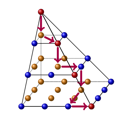
# #### Graphic representation
#
#
#
# [https://youtu.be/E1T1AWcMDqE](https://youtu.be/E1T1AWcMDqE)
#
# Description: Linear programming and optimal transport problems.
# ### Linear programming
#
# - Finding maximum/minimum of linear function subject to a set of linear inequality constraints
# - Classical problem in operations research and economics
#
#
# **Optimal transport problem**
#
# Minimum cost of transporting a set of goods from $ m $ origins to $ n $ destinations,
# where cost of transporting from origin $ i $ to destination $ j $ is given by $ c_{ij} $
# ### Optimal transport in economics
#
# - Matching and trade
# - matching distribution of workers to distribution of firms
# - relation to gravity equation in trade
# - Demand estimation and pricing
# - relation to discrete choice and nested discrete choice
# - quasi-linear hedonic models
# - Quantile methods in econometrics
# #### Graphic representation
#
#  # #### Formal problem statement
#
# $$
# \min \sum_{i=1}^{m}\sum_{j=1}^{n} c_{ij} x_{ij}, \text{ subject to}
# $$
#
# $$
# \sum_{i=1}^{m} x_{ij} = b_j, j \in \{1,\dots,n\},
# $$
#
# $$
# \sum_{j=1}^{n} x_{ij} = a_i, i \in \{1,\dots,m\},
# $$
#
# $$
# x_{ij} \ge 0 \text{ for all } i,j
# $$
# #### General linear programming problem
#
# Linear programming = optimizing linear function on convex polyhedron
#
# $$
# \max(c \cdot x) \text{ subject to } Ax \le b
# $$
#
# Note that $ Ax \le b $ includes as special cases
#
# - $ x_j\ge 0 $ for some $ j \in J $, trivially
# - $ x_j = D_j $ for some $ j \in J $ using two inequalities
# #### Convex polyhedron in 2d (convex polygon)
#
#
# #### Formal problem statement
#
# $$
# \min \sum_{i=1}^{m}\sum_{j=1}^{n} c_{ij} x_{ij}, \text{ subject to}
# $$
#
# $$
# \sum_{i=1}^{m} x_{ij} = b_j, j \in \{1,\dots,n\},
# $$
#
# $$
# \sum_{j=1}^{n} x_{ij} = a_i, i \in \{1,\dots,m\},
# $$
#
# $$
# x_{ij} \ge 0 \text{ for all } i,j
# $$
# #### General linear programming problem
#
# Linear programming = optimizing linear function on convex polyhedron
#
# $$
# \max(c \cdot x) \text{ subject to } Ax \le b
# $$
#
# Note that $ Ax \le b $ includes as special cases
#
# - $ x_j\ge 0 $ for some $ j \in J $, trivially
# - $ x_j = D_j $ for some $ j \in J $ using two inequalities
# #### Convex polyhedron in 2d (convex polygon)
#
#  # #### Convex polyhedron and objective function
#
#
# #### Convex polyhedron and objective function
#
#  # #### Convex polyhedron in 3d
#
#
# #### Convex polyhedron in 3d
#
#  # #### Example: Optimal production portfolio
#
# Let $ x $ and $ y $ denote production of goods A and B by some firm. The production technology is restricted to have
#
# $$
# \begin{cases}
# y - x &\le& 4, \\
# 2x - y &\le&8,
# \end{cases}
# $$
#
# And the resource constraint is given by $ x + 2y \le 14 $
#
# Let profits be given by $ \pi(x,y) = y + 2x $
# Adding the natural non-negativity constraints, in matrix notation we have
#
# $$
# \max(c^{T}x) \text{ subject to } Ax \le b
# $$
#
# $$
# c=
# \begin{pmatrix}
# 2 & 1
# \end{pmatrix},\;\;
# A=
# \begin{pmatrix}
# -1 & 1 \\
# 2 & -1 \\
# 1 & 2 \\
# -1 & 0 \\
# 0 & -1 \\
# \end{pmatrix},\;\;
# b=
# \begin{pmatrix}
# 4\\
# 8\\
# 14\\
# 0\\
# 0
# \end{pmatrix}
# $$
# #### Convex polyhedron and objective function
#
#
# #### Example: Optimal production portfolio
#
# Let $ x $ and $ y $ denote production of goods A and B by some firm. The production technology is restricted to have
#
# $$
# \begin{cases}
# y - x &\le& 4, \\
# 2x - y &\le&8,
# \end{cases}
# $$
#
# And the resource constraint is given by $ x + 2y \le 14 $
#
# Let profits be given by $ \pi(x,y) = y + 2x $
# Adding the natural non-negativity constraints, in matrix notation we have
#
# $$
# \max(c^{T}x) \text{ subject to } Ax \le b
# $$
#
# $$
# c=
# \begin{pmatrix}
# 2 & 1
# \end{pmatrix},\;\;
# A=
# \begin{pmatrix}
# -1 & 1 \\
# 2 & -1 \\
# 1 & 2 \\
# -1 & 0 \\
# 0 & -1 \\
# \end{pmatrix},\;\;
# b=
# \begin{pmatrix}
# 4\\
# 8\\
# 14\\
# 0\\
# 0
# \end{pmatrix}
# $$
# #### Convex polyhedron and objective function
#
#  # In[1]:
import numpy as np
from scipy.optimize import linprog
c = np.array([-2,-1])
A = np.array([[-1,1],[2,-1],[1,2],[-1,0],[0,-1]])
b = np.array([4,8,14,0,0])
def outf(arg):
print('iteration %d, current solution %s'%(arg.nit,arg.x))
linprog(c=c,A_ub=A,b_ub=b,method='simplex',callback=outf)
# ### Further learning resources
#
# - “Optimal Transport Methods in Economics” by Alfred Galichon, 2016
# [https://www.jstor.org/stable/j.ctt1q1xs9h](https://www.jstor.org/stable/j.ctt1q1xs9h)
# - Alfred Galichon’s plenary talk at the 2020 Econometric Society World Congress
# [https://youtu.be/XYIRkSIExik?t=2256](https://youtu.be/XYIRkSIExik?t=2256)
# In[1]:
import numpy as np
from scipy.optimize import linprog
c = np.array([-2,-1])
A = np.array([[-1,1],[2,-1],[1,2],[-1,0],[0,-1]])
b = np.array([4,8,14,0,0])
def outf(arg):
print('iteration %d, current solution %s'%(arg.nit,arg.x))
linprog(c=c,A_ub=A,b_ub=b,method='simplex',callback=outf)
# ### Further learning resources
#
# - “Optimal Transport Methods in Economics” by Alfred Galichon, 2016
# [https://www.jstor.org/stable/j.ctt1q1xs9h](https://www.jstor.org/stable/j.ctt1q1xs9h)
# - Alfred Galichon’s plenary talk at the 2020 Econometric Society World Congress
# [https://youtu.be/XYIRkSIExik?t=2256](https://youtu.be/XYIRkSIExik?t=2256)