#!/usr/bin/env python
# coding: utf-8

# # Python Boot Camp
# 
# **Lecturer**: None<br>
# **Jupyter Notebook Author**: Leo Singer, Cameron Hummels, Igor Andreoni
# 
# This is a Jupyter notebook lesson taken from the GROWTH Summer School 2020.  For other lessons and their accompanying lectures, please see: http://growth.caltech.edu/growth-school-2020.html
# 
# ## Objective
# Introduce the user to basic usage of Python.  Includes some basic analysis of photometric data using astropy.
# 
# ## Key steps
# - Variable manipulation
# - Lists, arrays, floats, ints, sets, dictionaries
# - Conditionals, loops
# - Error handling
# - Intro to numpy
# - Intro to astropy
# 
# ## Required dependencies
# 
# See GROWTH school webpage for detailed instructions on how to install these modules and packages.  Nominally, you should be able to install the python modules with `pip install <module>`.  The external astromatic packages are easiest installed using package managers (e.g., `rpm`, `apt-get`).
# 
# ### Python modules
# * python 3
# * astropy
# * numpy
# * matplotlib
# 
# ### External packages
# None

# ## I. Introduction
# 
# This workshop is about doing astronomical data analysis with the [Python programming language](https://python.org/). **No previous experience with Python is necessary!**
# 
# Python is a powerful tool, but it comes into its own as a numerical and data analysis environment with the following packages, which you will definitely want to have:
# 
# * **[Matplotlib](https://matplotlib.org)**: plotting interactive or publication-quality figures
# * **[Numpy](http://www.numpy.org)**: vectorized arithmetic and linear algebra
# * **[Scipy](https://www.scipy.org)**: curated collection of algorithms for root finding, interpolation, integration, signal processing, statistics, linear algebra, and much more
# * **[Jupyter Notebook](https://jupyter.org)** (formerly IPython Notebook): the Mathematica-like interface that you are using now, and last but not least
# * **[Astropy](https://www.astropy.org/)**: a community library for astronomy.
# 
# We'll cover the basics of Python itself and then dive in to some applications to explore each of these packages.

# **NOTE:** The purest way of interacting with Python is via its command line interpreter, which looks like this:
# 
# ![A session in the Python command line interpreter](https://raw.github.com/lpsinger/astropy-tutorial/master/terminal.png)

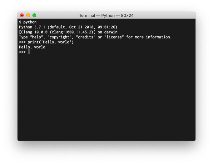
# A relatively new but very powerful way of using Python is through the Jupyter Notebook interface, which like Mathematica allows you to intermingle computer code with generated plots.  You're using one now.

# In[ ]:


from matplotlib import pyplot as plt
import numpy as np
get_ipython().run_line_magic('matplotlib', 'inline')

x = np.linspace(0, 2 * np.pi)
plt.plot(x, np.sin(x))
plt.xlabel('ppm caffeine in bloodstream')
plt.ylabel('cheeriness')


# and tables...

# In[ ]:


import astropy.table
tbl = astropy.table.Table()
tbl.add_column(astropy.table.Column(data=np.arange(5),
    name='integers'))
tbl.add_column(astropy.table.Column(data=np.arange(5)**2,
    name='their squares'))
tbl


# and even notes and typeset mathematics...
# 
# > *And God said:*
# >
# > > $$\nabla \cdot \mathbf{D} = \rho$$
# > > $$\nabla \cdot \mathbf{B} = 0$$
# > > $$\nabla \times \mathbf{E} = -\frac{\partial\mathbf{B}}{\partial t}$$
# > > $$\nabla \times \mathbf{H} = J + \frac{\partial\mathbf{D}}{\partial t}$$
# >
# > *and there was light.*
# 
# This is all very useful for doing interactive data analysis, so we will use the IPython Notebook interface for this tutorial. **WARNING:** I'm spoiling you rotten by doing this.

# ## II. How to get Python/Matplotlib/Numpy/Scipy/Astropy (if necessary)
# 
# Python and all of the packages that we discuss in this tutorial are open source software, so there multiple options for installing them.  <b>But if you followed the instructions on the GROWTH website for downloading/installing these modules, you have already installed these dependencies.  Skip to the next step.</b>

# ### For Linux/UNIX users
# 
# If you have one of the common Linux/UNIX distros (for example, [Ubuntu](https://www.ubuntu.com), [Debian](https://debian.org), or [Fedora](https://fedoraproject.org)), then you probably already have Python and you can get Matplotlib and friends from your package manager.
# 
# For example, on Debian or Ubuntu, use:
# 
#     $ sudo apt-get install jupyter-notebook python3-matplotlib python3-astropy python3-scipy

# ### For Mac users
# 
# Every version of Mac OS comes with a Python interpreter, but it's slightly easier to obtain Matplotlib and Numpy if you use a package manager such as [MacPorts](https://macports.org), [HomeBrew](https://brew.sh), or [Fink](http://www.finkproject.org). I use MacPorts (and contribute to it, too), so that's what I suggest. Install MacPorts and then do:
# 
#     $ sudo port install py37-matplotlib py37-scipy py37-jupyterlab py37-astropy

# ### For Windows users
# 
# Windows does not come with Python, but popular and free builds of Python for Windows include [Anaconda](https://www.anaconda.com/distribution/) and [Canopy](https://www.enthought.com/product/canopy/). Another alternative for Windows is to set up a virtual machine with [VirtualBox](https://www.virtualbox.org) and then install a Linux distribution on that.

# ## III. Python basics

# ### The `print()` function and string literals

# If this is your first time looking at Python code, the first thing that you might notice is that it is very easy to understand. For example, to print something to the screen, it's just:

# In[ ]:


print('Hello world!')


# This is a Python statement, consisting of the built-in command `print` and a string surrounded by single quotes. Double quotes are fine inside a string:

# In[ ]:


print('She said, "Hello, world!"')


# But if you want single quotes inside your string, you had better delimit it with double quotes:

# In[ ]:


print("She said, 'Hello, world!'")


# If you need both single quotes and double quotes, you can use backslashes to escape characters.

# In[ ]:


print('She said, "O brave new world, that has such people in\'t!"')


# If you need a string that contains newlines, use triple quotes (`'''`) or triple double quotes (`"""`):

# In[ ]:


print("""MIRANDA
  O, wonder!
  How many goodly creatures are there here!
  How beauteous mankind is! O brave new world
  That has such people in't!""")


# Let's say that you need to print a few different things on the same line. Just separate them with commas, as in:

# In[ ]:


person = 'Miranda'
print("'Tis new to", person)


# Oops. I'm getting ahead of myself—you've now seen your first variable assignment in Python. Strings can be concatened by adding them:

# In[ ]:


'abc' + 'def'


# Or repeated by multiplying them:

# In[ ]:


'abcdef' * 2


# ### Numeric and boolean literals

# Python's numeric types include integers and both real and complex floating point numbers:

# In[ ]:


a = 30 # an integer
b = 0xDEADBEEF # an integer in hexadecimal
c = 3.14159 # a floating point number
d = 5.1e10 # scientific notation
e = 2.5 + 5.3j # a complex number
hungry = True # boolean literal
need_coffee = False # another boolean literal


# By the way, all of the text on a given line after the trailing hash sign (`#`) is a comment, ignored by Python.
# 
# The arithmetic operators in Python are similar to C, C++, Java, and so on. There is addition (and subtraction):

# In[ ]:


a + c


# Multiplication:

# In[ ]:


a * e


# Division:

# In[ ]:


a / c


# ***Important note***: unlike C, C++, Java, etc., ***division of integers gives you floats***:

# In[ ]:


7 / 3


# If you want integer division, then use the double-slash `//` operator:

# In[ ]:


a = 7
b = 3
7 // 3


# The `%` sign is the remainder operator:

# In[ ]:


32 % 26


# Exponentiation is accomplished with the `**` operator:

# In[ ]:


print(5 ** 3, 9**-0.5)


# ### Tuples

# A tuple is a sequence of values. It's just about the handiest thing since integers. A tuple is immutable: once you have created it, you cannot add items to it, remove items from it, or change items. Tuples are very handy for storing short sequences of related values or returning multiple values from a function. This is what tuples look like:

# In[ ]:


some_tuple = ('a', 'b', 'c')
another_tuple = ('caffeine', 6.674e-11, 3.14, 2.718)
nested_tuple = (5, 4, 3, 2, ('a', 'b'), 'c')


# Once you have made a tuple, you might want to retrieve a value from it. You index a tuple with square brackets, ***starting from zero***:

# In[ ]:


some_tuple[0]


# In[ ]:


some_tuple[1]


# You can access whole ranges of values using ***slice notation***:

# In[ ]:


nested_tuple[1:4]


# Or, to count backward from the end of the tuple, use a ***negative index***:

# In[ ]:


another_tuple[-1]


# In[ ]:


another_tuple[-2]


# Strings can be treated just like tuples of individual charaters:

# In[ ]:


person = 'Miranda'
print(person[3:6])


# ### Lists

# What if you want a container like a tuple but to which you can add or remove items or alter existing items? That's a list. The syntax is almost the same, except that you create a list using square brackets `[]` instead of round ones `()`:

# In[ ]:


your_list = ['foo', 'bar', 'bat', 'baz']
my_list = ['xyzzy', 1, 3, 5, 7]


# But you can change elements:

# In[ ]:


my_list[1] = 2
print(my_list)


# Or append elements to an existing list:

# In[ ]:


my_list.append(11)
print(my_list)


# Or delete elements:

# In[ ]:


del my_list[0]
print(my_list)


# ### Sets

# Sometimes you need a collection of items where order doesn't necessarily matter, but each item is guaranteed to be unique. That's a set, created just like a list or tuple but with curly braces `{}`:

# In[ ]:


a = {5, 6, 'foo', 7, 7, 8}
print(a)


# You can add items to a set:

# In[ ]:


a.add(3)
print(a)


# Or take them away:

# In[ ]:


a.remove(3)
print(a)


# You also have set-theoretic intersections with the `&` operator:

# In[ ]:


{1, 2, 3, 4, 5, 6} & {3, 4}


# And union with the `|` operator:

# In[ ]:


{1, 2, 3, 4, 5, 6} | {6, 7}


# And set difference with the `-` operator:

# In[ ]:


{1, 2, 3, 4, 5, 6} - {3, 4}


# ### Dictionaries

# Sometimes, you want a collection that is like a list, but whose indices are strings or other Python values. That's a dictionary. Dictionaries are handy for any type of database-like operation, or for storing mappings from one set of values to another. You create a dictionary by enclosing a list of key-value pairs in curly braces:

# In[ ]:


my_grb = {'name': 'GRB 130702A', 'redshift': 0.145, 'ra': (14, 29, 14.78), 'dec': (15, 46, 26.4)}
my_grb


# You can index items in dictionaries with square braces `[]`, similar to tuples or lists:

# In[ ]:


my_grb['dec']


# or add items to them:

# In[ ]:


my_grb['url'] = 'http://gcn.gsfc.nasa.gov/other/130702A.gcn3'
my_grb


# or delete items from them:

# In[ ]:


del my_grb['url']
my_grb


# Dictionary keys can be any **immutable** kind of Python object: tuples, strings, integers, and floats are all fine. Values in a dictionary can be **any Python value at all**, including lists or other dictionaries:

# In[ ]:


{
    'foods': ['chicken', 'veggie burger', 'banana'],
    'cheeses': {'muenster', 'gouda', 'camembert', 'mozarella'},
    (5.5, 2): 42,
    'plugh': 'bat'
}


# ### The `None` object

# Sometimes you need to represent the absence of a value, for instance, if you have a gap in a dataset. You might be tempted to use some special value like `-1` or `99` for this purpose, but **don't**! Use the built-in object `None`.

# In[ ]:


a = None


# ### Conditionals

# In Python, control flow statements such as conditionals and loops have blocks indicated with indentation. Any number of spaces or tabs is fine, as long as you are consistent within a block. Common choices include four spaces, two spaces, or a tab.
# 
# You can use the `if`...`elif`...`else` statement to have different bits of code run depending on the truth or falsehood of boolean expressions. For example:

# In[ ]:


a = 5

if a < 3:
    print("i'm in the 'if' block")
    messsage = 'a is less than 3'
elif a == 3:
    print("i'm in the 'elif' block")
    messsage = 'a is 3'
else:
    print("i'm in the 'else' block")
    message = 'a is greater than 3'

print(message)


# You can chain together inequalities just like in mathematical notation:

# In[ ]:


if 0 < a <= 5:
    print('a is greater than 0 but less than or equal to 5')


# You can also combine comparison operators with the boolean `and`, `or`, and `not` operators:

# In[ ]:


if a < 6 or a > 8:
    print('yahoo!')


# In[ ]:


if a < 6 and a % 2 == 1:
    print('a is an odd number less than 6!')


# In[ ]:


if not a == 5: # same as a != 5
    print('a is not 5')


# The comparison operator `is` tests whether two Python values are not only equal, but represent the same object. Since there is only one `None` object, the `is` operator is particularly useful for detecting `None`.

# In[ ]:


food = None

if food is None:
    print('No, thanks')
else:
    print('Here is your', food)


# Likewise, there is an `is not` operator:

# In[ ]:


if food is not None:
    print('Yum!')


# The `in` and `not in` operators are handy for testing for membership in a string, set, or dictionary:

# In[ ]:


if 3 in {1, 2, 3, 4, 5}:
    print('indeed it is')


# In[ ]:


if 'i' not in 'team':
    print('there is no "i" in "team"')


# When referring to a dictionary, the `in` operator tests if the item is among the **keys** of the dictionary.

# In[ ]:


d = {'foo': 3, 'bar': 5, 'bat': 9}
if 'foo' in d:
    print('the key "foo" is in the dictionary')


# ### The `for` and `while` loops

# In Python, there are just two types of loops: `for` and `while`. `for` loops are useful for repeating a set of statements for each item in a collection (tuple, set, list, dictionary, or string). `while` loops are not as common, but can be used to repeat a set of statements until a boolean expression becomes false.

# In[ ]:


for i in [0, 1, 2, 3]:
    print(i**2)


# The built-in function `range`, which returns a list of numbers, is often handy here:

# In[ ]:


for i in range(4):
    print(i**2)


# Or you can have the range start from a nonzero value:

# In[ ]:


for i in range(-2, 4):
    print(i**2)


# You can iterate over the keys and values in a dictionary with `.items()`:

# In[ ]:


for key, val in d.items():
    print(key, '...', val**3)


# The syntax of the `while` loop is similar to the `if` statement:

# In[ ]:


a = 1
while a < 5:
    a = a * 2
    print(a)


# ### List comprehensions

# Sometimes you need a loop to create one list from another. List comprehensions make this very terse. For example, the following `for` loop:

# In[ ]:


a = []
for i in range(5):
    a.append(i * 10)


# is equivalent to this list comprehension:

# In[ ]:


a = [i * 10 for i in range(5)]


# You can even incorporate conditionals into a list comprehension. The following:

# In[ ]:


a = []
for i in range(5):
    if i % 2 == 0:
        # i is even
        a.append(i * 10)


# can be written as:

# In[ ]:


a = [i * 10 for i in range(5) if i % 2 == 0]


# ### Conditional expressions

# Conditional expressions are a closely related shorthand. The following:

# In[ ]:


if 6/2 == 3:
    a = 'foo'
else:
    a = 'bar'


# is equivalent to:

# In[ ]:


a = 'foo' if 6/2 == 3 else 'bar'


# ### Functions

# Functions are created with the `def` statement. A function may either have or not have a `return` statement to send back a return value.

# In[ ]:


def square(n):
    return n * n

a = square(3)
print(a)


# If you want to return multiple values from a function, return a tuple. Parentheses around the tuple are optional.

# In[ ]:


def powers(n):
    return n**2, n**3

print(powers(3))


# If a function returns multiple values, you can automatically unpack them into multiple variables:

# In[ ]:


square, cube = powers(3)
print(square)


# If you pass a mutable value such as a list to a function, then **the function may modify that value**. For example, you might implement the Fibonacci sequence like this:

# In[ ]:


def fibonacci(seed, n):
    while len(seed) < n:
        seed.append(seed[-1] + seed[-2])
    # Note: no return statement

seed = [1, 1]
fibonacci(seed, 10)
print(seed)


# You can also give a function's arguments default values, such as:

# In[ ]:


def fibonacci(seed, n=6):
    while len(seed) < n:
        seed.append(seed[-1] + seed[-2])
    # Note: no return statement

seed = [1, 1]
fibonacci(seed)
print(seed)


# If a function has a large number of arguments, it may be easier to read if you pass the arguments by keyword, as in:

# In[ ]:


seq = [1, 1]
fibonacci(seed=seq, n=4)


# ## IV. The Python standard library

# Python comes with an extensive **[standard library](http://docs.python.org/2/library/index.html)** consisting of individual **modules** that you can opt to use with the `import` statement. For example:

# In[ ]:


import math
math.sqrt(3)


# In[ ]:


from math import pi
pi


# Some particularly useful parts of the Python standard library are:
# 
# * [`random`](https://docs.python.org/3/library/random.html): random number generators
# * [`pickle`](https://docs.python.org/3/library/pickle.html): read/write Python objects into files
# * [`sqlite3`](https://docs.python.org/3/library/sqlite3.html): SQLite database acces
# * [`os`](https://docs.python.org/3/library/os.html): operating system services
# * [`os.path`](https://docs.python.org/3/library/os.path.html): file path manipulation
# * [`subprocess`](https://docs.python.org/3/library/subprocess.html): launch external processes
# * [`email`](https://docs.python.org/3/library/email.html): compose, parse, receive, or send e-mail
# * [`pdb`](https://docs.python.org/3/library/pdb.html): built-in debugger
# * [`re`](https://docs.python.org/3/library/re.html): regular expressions
# * [`http`](https://docs.python.org/3/library/http.html): built-in lightweight web client and server
# * [`optparse`](https://docs.python.org/3/library/optparse.html): build pretty command-line interfaces
# * [`itertools`](https://docs.python.org/3/library/itertools.html): exotic looping constructs
# * [`multiprocessing`](https://docs.python.org/3/library/multiprocessing.html): parallel processing

# ### Error handling

# It can be important for your code to be able to handle error conditions. For example, let's say that you are implementing a sinc function:

# In[ ]:


def sinc(x):
    return math.sin(x) / x

print(sinc(0))


# Oops! We know that by definition $\mathrm{sinc}(0) = 1$ , so we should catch this error:

# In[ ]:


def sinc(x):
    try:
        result = math.sin(x) / x
    except ZeroDivisionError:
        result = 1
    return result

print(sinc(0))


# ### Reading and writing files

# The built-in `open` function opens a file and returns a `file` object that you can use to read or write data. Here's an example of writing data to a file:

# In[ ]:


myfile = open('myfile.txt', 'w') # open file for writing
myfile.write("red 1\n")
myfile.write("green 2\n")
myfile.write("blue 3\n")
myfile.close()


# And here is reading it:

# In[ ]:


d = {} # create empty dictionary

for line in open('myfile.txt', 'r'): # open file for reading
    color, num = line.split() # break apart line by whitespace
    num = int(num) # convert num to integer
    d[color] = num

print(d)


# ## V. Numpy & Matplotlib

# Numpy provides array operations and linear algebra to Python. A Numpy array is a bit like a Python list, but supports elementwise arithmetic. For example:

# In[ ]:


import numpy as np

x = np.asarray([1, 2, 3, 4, 5])
y = 2 * x
print(y)


# Numpy arrays may have any number of dimensions:

# In[ ]:


x = np.asarray([[1, 2, 3], [4, 5, 6], [7, 8, 9]])
x


# In[ ]:


y = np.asarray([[9, 8, 7], [6, 5, 4], [3, 2, 1]])
y


# An array has a certain number of dimensions denoted `.ndim`:

# In[ ]:


x.ndim


# and the dimensions' individual lengths are given by `.shape`:

# In[ ]:


x.shape


# and the total number of elements by `.size`:

# In[ ]:


x.size


# By default, multiplication is elementwise:

# In[ ]:


x * y


# To perform matrix multiplication, either convert arrays to `np.matrix` or use `np.dot`:

# In[ ]:


np.asmatrix(x) * np.asmatrix(y)


# In[ ]:


np.dot(x, y)


# You can also perform comparison operations on arrays...

# In[ ]:


x > 5


# Although a boolean array doesn't directly make sense in an `if` statement:

# In[ ]:


if x > 5:
    print('oops')


# In[ ]:


if np.any(x > 5):
    print('at least some elements are greater than 5')


# You can use conditional expressions like indices:

# In[ ]:


x[x > 5] = 5
x


# Or manipulate individual rows:

# In[ ]:


x[1, :] = -1
x


# Or individual columns:

# In[ ]:


x[:, 1] += 100
x


# Other useful features include various random number generators:

# In[ ]:


from matplotlib import pyplot as plt
get_ipython().run_line_magic('matplotlib', 'inline')

# Plot histogram of 10k normal random variates
plt.hist(np.random.randn(10000))


# In[ ]:


np.random.uniform(low=0, high=2*np.pi)


# You've already seen a few examples of Matplotlib. If you have used MATLAB, then Matplotlib code may look familiar.

# In[ ]:


x = np.linspace(-10, 10)
y = 1 / (1 + np.exp(x))
plt.plot(x, y)
plt.annotate(
    'foo bar', (x[20], y[20]), (50, 5),
    textcoords='offset points',
    arrowprops={'arrowstyle': '->'})
plt.grid()


# ****
# # BREAKOUT SESSION 1
# 
# Test exercise: plot up your name, or the initial(s) of your name. Get creative!
# There is not a 'right way' or a 'wrong way' to do this exercise, but try not to use plt.text() or plt.annotate(). Too easy. :-)

# In[ ]:


...


# ****

# ## VI. Astropy

# Astropy is a core Python package for astronomy. It is formed from the merger of a number of other Python astronomy packages, but also contains a lot of original code. Core features include:
# 
# * `astropy.constants`, `astropy.units`: Physical constants, units, and unit conversion
# * `astropy.time`: Manipulation of dates and times
# * `astropy.coordinates`: Representation of and conversion between astronomical coordinate systems
# * `astropy.table`: Tables and gridded data
# * `astropy.io.fits`: Manipulating FITS files
# * `astropy.io.ascii`: Manipulating ASCII tables of many different formats
# * `astropy.io.votable`: Virtual Observatory tables
# * `astropy.wcs`: World Coordinate System transformations
# * `astropy.cosmology`: Cosmological calculations
# * `astropy.stats`: Astrostatistics
# * `astropy.modeling`: multi-D model fitting Swiss army knife
# 
# The Astropy project also has sevearl ["affiliated packages"](http://www.astropy.org/affiliated/index.html) that have similar design but are maintained separately, including:
# 
# * [Photutils](https://photutils.readthedocs.io/): Aperture photometry
# * [Astroquery](https://astroquery.readthedocs.io/): Query astronomical databases

# Astropy will be used extensively during the course of the school.

# ****
# # BREAKOUT SESSION 2
# 
# On August 17th 2017, a bright kilonova was found during the follow-up of the gravitational wave event GW170817. More than 70 telescopes around the world managed to observe the transient at almost every wavelength.
# 
# We prepared a file with some optical and near-infrared photometric data of the GW170817 kilonova. This dataset was taken from:
# - Arcavi et al.; Nature, Volume 551, Issue 7678, pp. 64-66 (2017).
# - Kasliwal et al.; Science, Volume 358, Issue 6370, pp. 1559-1565 (2017)
# 
# A compilation of existing datasets can be found at https://kilonova.space/kne/GW170817/
# 
# **Exercise:** plot the optical/near-infrared light curve of GW170817

# In[ ]:


# Read the light curve file
from astropy.io import ascii

# Easier version: use a file that includes only g-band data
t = ascii.read("data/GW170817_Arcavi_Kasliwal_g.csv", format='csv')

# Pro version: use a file that includes multi-band data
#t = ascii.read("data/GW170817_Arcavi_Kasliwal_griJ.csv", format='csv')


# With the `astropy.ascii` class, we read the light curve as an `astropy` `Table` object. Run the next cell to display the table

# In[ ]:


t


# Plot!
# 
# - Tip 1: it can be convenient to use the plt.errorbar() method 
# - Tip 2: If you chose the multi-band file, you may want to iterate over a list (or set) of bands

# In[ ]:


# Define a dictionary for the colors (feel free to edit it)
colors = {'g': 'b', 'r': 'r', 'i': 'y', 'J': "orange"}

# Let's place the time axis origin when the binary merger occurred. Astropy can help with this.
from astropy.time import Time

time_merger = Time('2017-08-17 12:41:04.4', format='iso')
# Note that the times in the table are expressed as 'modified Julian dates (MJD)'
t["time_delta"] = t["time_mjd"] - time_merger.mjd

# Plot
...

plt.ylim(...)
plt.xlabel("Time from merger [days]")
plt.ylabel("Apparent magnitude (AB system)")

# Title, legend
...


# ****