#!/usr/bin/env python
# coding: utf-8
# # Jupyter Notebook Tutorial
# ## JHU Data Services
# ### Website: [dataservices.library.jhu.edu](https://dataservices.library.jhu.edu/)
# ### Contact: dataservices@jhu.edu
# This interactive tutorial covers the basics of using Jupyter Notebooks with Python. It includes screenshots, written instructions, and practice questions to prepare participants to use Jupyter Notebooks in JHU Data Services workshops. Before using this notebook, make sure to install Anaconda on your computer. Installation instructions can be found in our [GitHub repository](https://github.com/jhu-data-services/python-installation-instructions).
# ## Sections in this notebook:
#
# - [Open a Jupyter Notebook using Anaconda](#Open-a-Jupyter-Notebook-using-Anaconda)
# - [Create a new notebook](#Create-a-new-notebook)
# - [Add and remove cells](#Add-and-remove-cells)
# - [Switch between code and markdown cell types](#Switch-between-code-and-markdown-cell-types)
# - [Run cells](#Run-cells)
# - [Format cells using Markdown syntax](#Format-cells-using-Markdown-syntax)
# - [Magic functions](#Magic-functions)
# - [Analyze and Visualize data](#Analyze-and-Visualize-data)
# - [Appendix](#Appendix)
#
#
#
#
#
# ## Open a Jupyter Notebook using Anaconda
# This tutorial uses the [Anaconda Individual Edition](https://www.anaconda.com/products/individual) to take advantage of the graphical user interface (GUI) to install and run Jupyter Notebooks. The Jupyter Notebook software can also be installed directly from [Project Jupyter](https://jupyter.org/install) and can be run using the command line.
#
# After you have installed Anaconda Individual Edition (see the [installation page](https://www.anaconda.com/products/individual) and [user guide](https://docs.anaconda.com/anaconda/user-guide/) for more information), open the __Anaconda Navigator:__
# 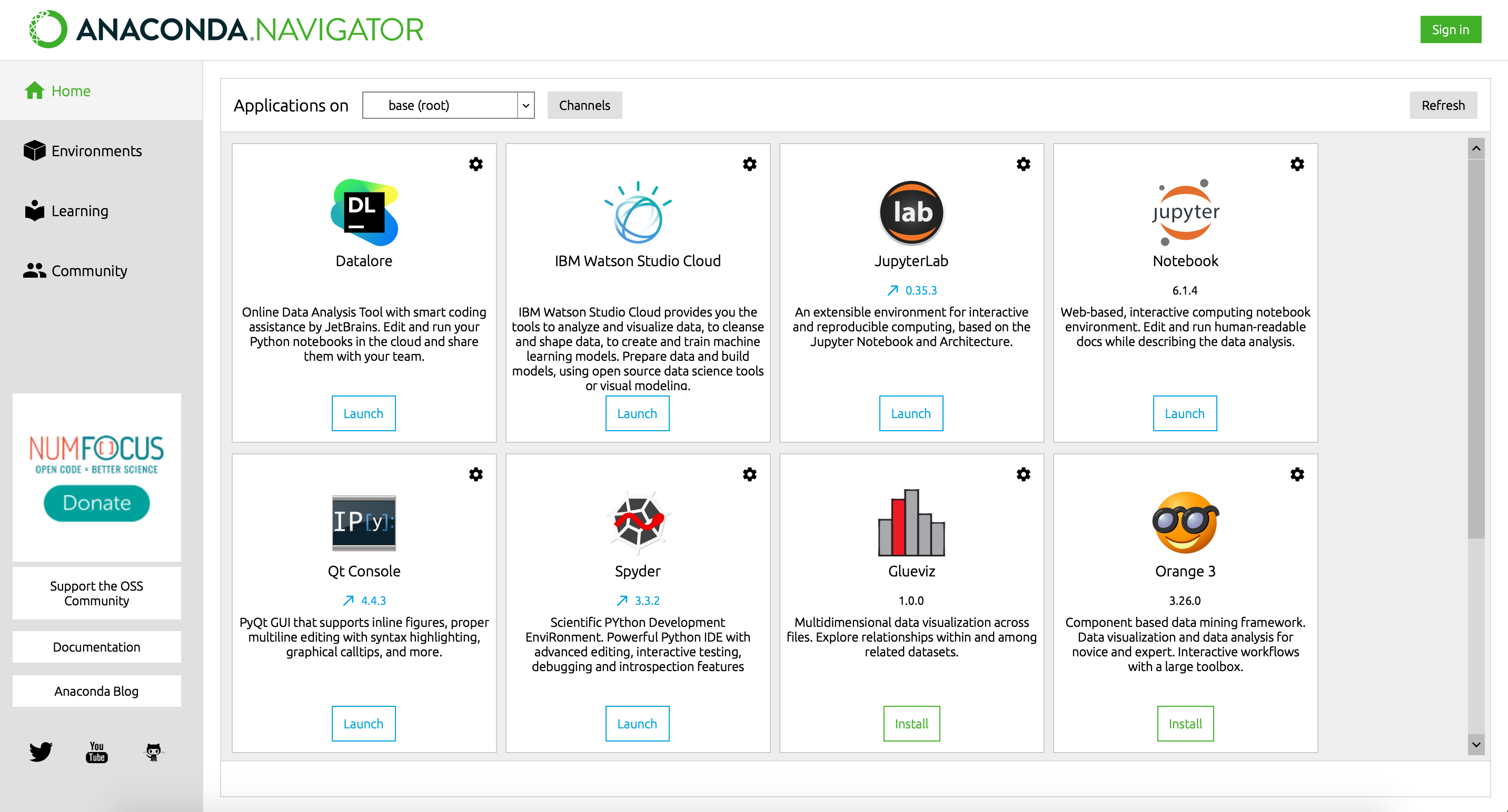
# _Note: your version of Navigator might look different depending on version updates. You may also have different versions of the available applications._
# To open Jupyter Notebooks, navigate to the __Jupyter Notebook__ application (top-right box in the screenshot above) and click the blue __Launch__ button.
#
# Jupyter Notebooks will now open in a new tab in your default web browser. It will open to a file browser that looks like this:
# 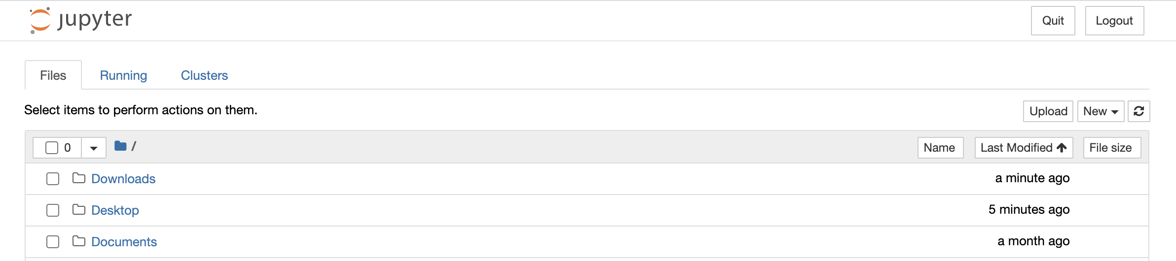
# Navigate to the directory where you want to create a new notebook (if opening an existing notebook, navigate to the directory where that notebook is saved). To open an existing notebook, click on the filename (file extension .ipynb). The notebook will open in a new tab in your web browser.
# ## Create a new notebook
# To create a new notebook, click __New__ in the upper-right corner. Choose your kernel, or programming language, from the drop-down menu. This tutorial will use Python 3.
# 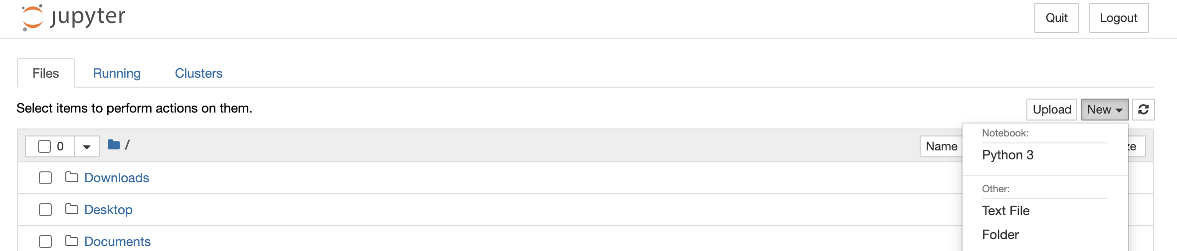
# This will open your new notebook in a new tab in your browser.
#
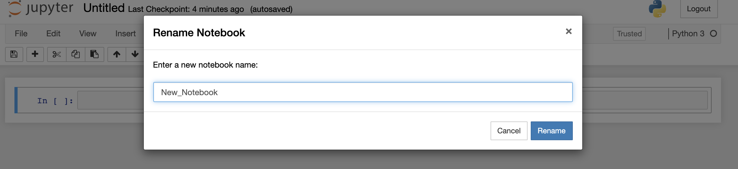
# Start by giving your new notebook a descriptive title. Click the title at the top of the page (the default title is "Untitled") to rename your notebook. Type your new notebook name in the text box and click __Rename__.
# 
# ## Add and remove cells
# Your notebook starts with only one code cell. There are several ways to add more cells to a notebook:
# 1. Click the __+__ sign button in the toolbar at the top of your notebook.
# 2. Click the __Insert__ drop-down menu at the top of your notebook. Select __Insert Cell Above__ or __Insert Cell Below__ to add a new cell either above or below whichever cell is currently selected.
# 3. Use keyboard shortcuts: the __A__ key inserts a new cell above your current selection; the __B__ key inserts a new cell below your current selection.
#
# Try one of these methods to add a new cell below:
#
# To remove a cell, you can:
# 1. Click the button across the top with the scissors icon.
# 2. Click the __Edit__ drop-down menu and choose __Cut Cells__ or __Delete Cells__ to remove a selected cell.
# 3. Use the keyboard shortcut __X__ to cut a cell or __DD__ (press the D key twice) to delete a selected cell.
#
# *Note: The* **cut** *function will remove a cell and copy it, making it available to paste elsewhere in your notebook. The* **delete** *function will remove a cell without copying it.*
#
# Try one of these methods to remove the cell below:
# In[ ]:
# remove this cell
# ## Switch between code and markdown cell types
# When working with your notebook, you will likely want a mix of code cells, written in Python, and markdown cells, with narrative text to explain your analysis and results.
#
# When creating a new cell, the default cell type is Code. You can change the cell type by clicking the drop-down menu along the top that says __Code__. When the cell is selcted, change the type to __Markdown__ using the menu.
#
# Change a markdown cell back to code using the same method. The drop-down menu will say __Markdown__ when a markdown cell is selected. Click the menu and select __Code__ to change the cell type to code.
#
# You can also use keyboard shortcuts to change the type of a selected cell:
# The __M__ key changes a cell to Markdown
# The __Y__ key changes a cell to Code
#
# Use either method to change the code cell below to Markdown, and the markdown cell below to Code.
# In[ ]:
# change this cell to Markdown
# Change this cell to Code
# ## Run cells
# Just as with creating and removing cells, there are several ways to run a cell in a Jupyter Notebook:
# 1. Click the __Run__ button in the toolbar at the top of your notebook.
# 2. Use the __Cell__ drop-down menu to choose an option:
# 1. Run Cells - runs selected cell
# 2. Run Cells and Select (or Insert) Below - runs selected cell and selects (or inserts a new) cell below
# 3. Run All - runs all cells in the notebook
# 4. Run All Above (or Below) - runs all cells above (or Below) the selected cell
# 3. Use one of the keyboard shortcuts displayed next to each option in the __Cell__ drop-down menu (keyboard shortcuts are different on Windows vs. Mac).
#
# Use any of these options to run the next five cells. Notice that:
# - Cells can contain multiple lines of code
# - Notebooks are run interactively, so code executed in one cell affects the code executed in later cells
# - Code cells can contain comments, define functions, and more, just like other Python development environments
# In[ ]:
# define a function to add 1 to a numeric input
def add_one(num):
new_num = num + 1
return new_num
# In[ ]:
add_one(1)
# In[ ]:
three_plus_one = add_one(3)
# In[ ]:
three_plus_one
# In[ ]:
my_list = [1, 2, 3, 4, 5, 6, 7, 8, 9, 10]
for index, item in enumerate(my_list):
my_list[index] = add_one(item)
my_list # each element should have increased by 1
# When running cells in a Jupyter Notebook, make sure you are running them in the correct order!
#
# Notebooks should be designed to run from top to bottom, with all dependencies, libraries, and functions located at the top. This helps to avoid errors and makes sure there is no confusion about the order in which cells should be run.
# ## Format cells using Markdown syntax
# Jupyter Notebooks are a great tool for documenting and explaining your code through narrative text. To edit this text, Jupyter Notebooks use Markdown, a lightweight markup language for formatting plain text.
# Common markdown elements for Jupyter Notebooks:
#
# Element | Markdown Syntax
# :------- | :---------------
# Heading | `# H1`
`## H2`
`### H3`
(goes up to H6)
# Bold | `__two underscores__` or `**two asterisks**`
# Italic | `_one underscore_` or `*one asterisk*`
# Ordered list | `1. First item`
`2. Second item`
`3. Third item`
# Unordered list
(bullet points) | `- First item`
`- Second item`
`- Third item`
# Hyperlink | `[link name](URL)`
# Embed an image | ``
# Line break | Three spaces at the end of a line, or use the HTML `
` tag
# Add markdown syntax to format the text in the cells below:
# _Note: you may have to double-click each cell in order to edit it_
# Create a heading here
# Make this text bold
# Make a single word in this cell italic
# Create a list (ordered or unordered) for these items: "Complete Jupyter Notebooks tutorial," "Start using Jupyter Notebooks," "Become a reproducible research expert"
# Add a hyperlink to the JHU Data Services website: `https://dataservices.library.jhu.edu/`
# For more on Markdown and additional syntax for formatting plain text, see:
# - Markdown Guide - [markdownguide.org](https://www.markdownguide.org/)
# - Jupyter Notebook documentation - [Markdown Cells](https://jupyter-notebook.readthedocs.io/en/stable/examples/Notebook/Working%20With%20Markdown%20Cells.html#)
#
# You can also double-click any of the markdown cells in this document to see the syntax used to format each cell.
# ## Magic functions
# Magic functions, also called magic commands, are a component of IPython, the Jupyter kernel that allows you to use Python interactively within a Jupyter Notebook. Magic functions can help make your data analysis more efficient.
#
# The syntax to call a magic function is % for line magics, and %% for cell magics.
#
# You can learn more about magic functions from:
# - [The Python Data Science Handbook](https://jakevdp.github.io/PythonDataScienceHandbook/01.03-magic-commands.html)
# - [The IPython documentation on magic commands](https://ipython.readthedocs.io/en/stable/interactive/magics.html)
# - This article from [Towards Data Science](https://towardsdatascience.com/) titled [The Top 5 Magic Commands for Jupyter Notebooks](https://towardsdatascience.com/the-top-5-magic-commands-for-jupyter-notebooks-2bf0c5ae4bb8)
#
# _Note: Magic functions are part of the Python kernel and may not be available when using Jupyter Notebooks with other programming languages._
# In[ ]:
# run this cell to bring up documentation on magic functions
get_ipython().run_line_magic('magic', '')
# In[ ]:
# run this cell to list all of the available magic functions
get_ipython().run_line_magic('lsmagic', '')
# ## Analyze and Visualize data
# Jupyter Notebooks are a great tool for data analysis and visualization. Below is a sample workflow for importing a dataset, exploring data, and visualizing data. Feel free to add to this analysis or choose a new dataset to explore and visualize.
# This example uses data from the [Seaborn library](https://seaborn.pydata.org/), a data visualization library with 18 built-in datasets.
#
# This example will be using the `tips` dataset, which is a collection of tips received by a restaurant server. See all available datasets in the Seaborn library by importing the library and running `sns.get_dataset_names()` in a new code cell.
# ### Research question
# Is it better for this restaurant server to work a lunch shift or a dinner shift?
# ### Notebook setup
# You will need several libraries installed in order to run this analysis:
# - pandas
# - seaborn
# - matplotlib
#
# If you need to install any of these libraries, see the Anaconda documentation for [managing packages using the Navigator interface](https://docs.anaconda.com/anaconda/navigator/getting-started/#navigator-managing-packages) or this [tutorial for installing Pandas using Anaconda](https://docs.anaconda.com/anaconda/navigator/tutorials/pandas/).
#
# These packages can also be installed in a command-line interface using `pip` or `conda`.
# In[ ]:
# import required libraries
import pandas as pd
import seaborn as sns
from matplotlib import pyplot as plt
get_ipython().run_line_magic('matplotlib', 'inline')
# ### Create a dataframe
# In[ ]:
tips = sns.load_dataset('tips')
# ### Explore the dataframe
# The `tips` dataset was collected from a restaurant server's tips in 1990. See more about the dataset [on Kaggle](https://www.kaggle.com/ranjeetjain3/seaborn-tips-dataset).
#
# Data dictionary:
#
# Variable Name | Definition
# :-------: | :---------------:
# total_bill | total bill, in USD
# tip | added tip, in USD
# sex | sex of person paying for the meal (possible values: Male; Female)
# smoker | smoker in party? 0 = no, 1 = yes
# day | day of the week
# time | shift (possible values: Dinner; Lunch)
# size | size of the party
# In[ ]:
tips.head(10) # view the first 10 rows of the data
# In[ ]:
tips.dtypes # see the data type of each column
# In[ ]:
tips.shape # see the number of rows and columns in this dataframe
# Let's add a new column, tip_percent, that represents the percentage of the total bill that each customer tipped. Tip percentages will be rounded up to two decimal places.
# In[ ]:
tips['tip_percent'] = tips['tip'] / tips['total_bill']
tips['tip_percent'] = round(tips['tip_percent'], 2)
# In[ ]:
tips.head(10)
# ### Analyze and Visualize the data
# Let's start thinking about our research question: Is it better for this server to work a lunch shift or a dinner shift? There are many ways we could answer this question. For this analysis, we will look at which shift yields higher tip percentages, and which shift yields more tip money.
# #### Which shift yields higher tip percentages?
# In[ ]:
# create two new dataframes, one for lunch shift and one for dinner shift
lunch = tips[tips.time == 'Lunch']
dinner = tips[tips.time == 'Dinner']
# In[ ]:
# create histograms to visualize distribution of tip percentage for each shift
sns.set_style('ticks')
sns.displot(data=lunch, x='tip_percent')
plt.title('Distribution of tip percentages, Lunch shift')
# In[ ]:
sns.displot(data=dinner, x='tip_percent')
plt.title('Distribution of tip percentages, Dinner shift')
# We can plot these graphs on the same axes using the full `tips` dataset, to more closely compare distribution of tip percentage:
# In[ ]:
sns.displot(data=tips, x='tip_percent', hue='time', kind='kde')
plt.title('Distribution of tip percentages, Lunch and Dinner shifts')
# From these three graphs, we can see the majority of tips for both Lunch and Dinner shifts seem to be around 15%. Let's create a boxplot to compare these shifts more closely.
# In[ ]:
plt.figure(figsize=(18,8))
sns.set_theme(style='whitegrid')
sns.boxplot(data=tips, x='tip_percent', y='time')
plt.title('Distribution of tip percentages, Lunch and Dinner shifts')
# From the boxplots, we can see that the median tip percentage is higher during Dinner shift. Let's calculate the median percentages (50th percentile) and the mean tip percentage for each shift below.
# In[ ]:
# calculate tip percentage summary statistics for Lunch shift
lunch['tip_percent'].describe(percentiles=[.5])
# In[ ]:
# calculate tip percentage summary statistics for Dinner shift
dinner['tip_percent'].describe(percentiles=[.5])
# Looking at tip percentage, there does not seem to be a large difference between Lunch shift and Dinner shift. Though the median tip percentage for Dinner shift is higher (16% compared to 15% at Lunch shift), the mean tip percentage is slightly higher during Lunch shift (16.4% compared to 16% at Dinner shift).
# What might be more important than the percentage of each bill the server is being tipped, is the money the server is actually making in tips for each shift. Let's switch our focus to tip money, using the `tip` column of our dataset.
# #### Which shift yields higher tip money?
# In[ ]:
# visualize distribution of lunch and dinner tips
sns.set_style('ticks')
sns.displot(data=tips, x='tip', hue='time', kind='kde')
plt.title('Distribution of tip money, Lunch and Dinner shifts')
plt.xlabel('tip money ($)')
# At a glance, we can see that the majority of tips for Dinner shift seem to be just under 4.00 USD, while tips for Lunch shift peak closer to 2.00 USD.
# Once again, let's create boxplots to compare the distribution of tip money for each shift.
# In[ ]:
plt.figure(figsize=(18,8))
sns.set_theme(style='whitegrid')
sns.boxplot(data=tips, x='tip', y='time')
plt.title('Distribution of tip money, Lunch and Dinner shifts')
plt.xlabel('tip money ($)')
# In[ ]:
# calculate tip money summary statistics for Lunch shift
lunch['tip'].describe(percentiles=[.5])
# In[ ]:
# calculate tip money summary statistics for Lunch shift
dinner['tip'].describe(percentiles=[.5])
# We can see from the above boxplots and summary statistics that Dinner shift yields higher tip money on average (median and mean) than Lunch shift.
#
# Lunch shift yields a mean tip of **2.73 USD** per bill (median tip of 2.25 USD). Dinner shift yields a mean tip of **3.10 USD** per bill (median 3.00 USD).
# How can it be that this server gets higher tip percentages during Lunch shift, but makes more tip money during Dinner shift? One possible explanation is that dinner bills are higher than lunch bills. Let's look at total bill in USD:
# In[ ]:
# calculate summary statistics for total bill, Lunch shift
lunch['total_bill'].describe()
# In[ ]:
# calculate summary statistics for total bill, Dinner shift
dinner['total_bill'].describe()
# We can see from the summary statistics that our hypothesis is correct, customer bills during Dinner shift are higher on average (mean = 20.80 USD) than customer bills during Lunch shift (mean = 17.17 USD).
# #### Results: Which shift is better for this server?
# Based on the above analysis of tip percentage and tip money for Lunch and Dinner shifts, it seems that it is better for this server to work a Dinner shift, as they will make more tip money on average than working a Lunch shift.
# ***
# You have reached the end of this introductory tutorial.
#
# We hope you have become more comfortable with Jupyter Notebooks and understand how Jupyter Notebooks allow you to explore, analyze, and visualize data in an interactive and reproducible environment.
# ### About this tutorial
# This tutorial was created using Jupyter Notebooks version 6.1.4. Screenshots for using Anaconda and Jupyter Notebooks were taken in Anaconda Navigator version 1.10.0 and Jupyter Notebook version 6.1.4.
#
# ### Terms of Use
# This material is licensed under a [Creative Commons Attribution-NonCommercial 4.0 International License (CC BY-NC 4.0)](https://creativecommons.org/licenses/by-nc/4.0/) and may be shared for non-commerical purposes with proper attribution to the author. Please cite this material as:
#
# > Johns Hopkins University Data Services. (2021). Jupyter Notebook Tutorial. [https://github.com/jhu-data-services/python-installation-instructions/tree/main/jupyter-notebook-tutorial](https://github.com/jhu-data-services/python-installation-instructions/tree/main/jupyter-notebook-tutorial)
#
# The images and data used in this document may have other licensing and terms of use.
# ***
# ## Appendix
# Below are additional resources to help you make the most of Jupyter Notebooks.
# ### Jupyter Project documentation:
# [https://jupyter.readthedocs.io](https://jupyter.readthedocs.io/en/latest/)
# ### Jupyter Notebooks documentation:
# [https://jupyter-notebook.readthedocs.io](https://jupyter-notebook.readthedocs.io/en/latest/?badge=latest)
# ### Jupyter Notebook examples:
# [A Gallery of Interesting Jupyter Notebooks](https://github.com/jupyter/jupyter/wiki/A-gallery-of-interesting-Jupyter-Notebooks) on GitHub
# ### Common keyboard shortcuts:
# Shortcut | Function
# :-------: | :---------------:
# A | Insert cell above
# B | Insert cell below
# DD | Delete cell
# X | Cut cell
# Z | Undo delete or cut cell
# C | Copy cell
# V | Paste cell
# M | Change cell type to Markdown
# Y | Change cell type to Code