#!/usr/bin/env python
# coding: utf-8
# # Rician flat fading channel modeling
# ## (MATLAB tutorial)
# ### M.Sc. Vladimir Fadeev
# #### Kazan, 30.11.2018
# ## Preface
#
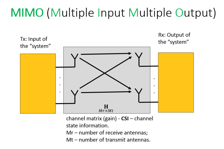
# Multiple Input Multiple Output (MIMO) system with linear arrays will be considered during this research.
#
# Why MIMO?
#
# Firstly, MIMO thechnology is the part of [LTE and LTE-A standards](https://gsmcommunications.blogspot.ru/2011/04/lte-long-term-evolution-phy-overview.html) that motivates us to learn little bit more about this.
#
# Moreover, we are considering MIMO system as the example of generalized communication system which can be easily simplified to more specific cases: MISO (Multiple Input Single Output), SIMO (Single Input Multiple Output) and SISO (Single Input Single Output).
#
# 
#
# More coplicated models should be researched for Massive MIMO technology (5G) and reqtangular antenna arrays cases.
# ## Introduction
# Let us start from the small theory explanation \[1, p. 11-12\]:
#
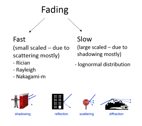
# > A signal propagating through the wireless channel arrives at the destination along a number of different paths, collectively referred to as multipath. These paths arise from scattering, reflection and diffraction of the radiated energy by objects in the environment or refraction in the medium. The different propagation mechanisms influence path loss and fading models differently. However, for convenience we refer to all these distorting mechanisms as “scattering”. Further, throughout the book, we assume a complex baseband representation for the signal and channel unless otherwise specified.
# >
# > The signal power drops off due to three effects: mean propagation (path) loss, macroscopic fading and microscopic fading. The mean propagation loss in macrocellular environments comes from inverse square law power loss, absorption by water and foliage and the effect of ground reflection. Mean propagation loss is range dependent.
# >
# > Macroscopic fading results from a blocking effect by buildings and natural features and is also known as long term fading or shadowing. Microscopic fading results from the constructive and destructive combination of multipaths and is also known as short term fading or fast fading. Multipath propagation results in the spreading of the signal in different dimensions. These are delay spread, Doppler (or frequency) spread (this needs a time-varying multipath channel) and angle spread. These spreads have significant effects on the signal. Mean path loss, macroscopic fading, microscopic fading, delay spread, Doppler spread and angle spread are the main channel effects and are described below.
#
# 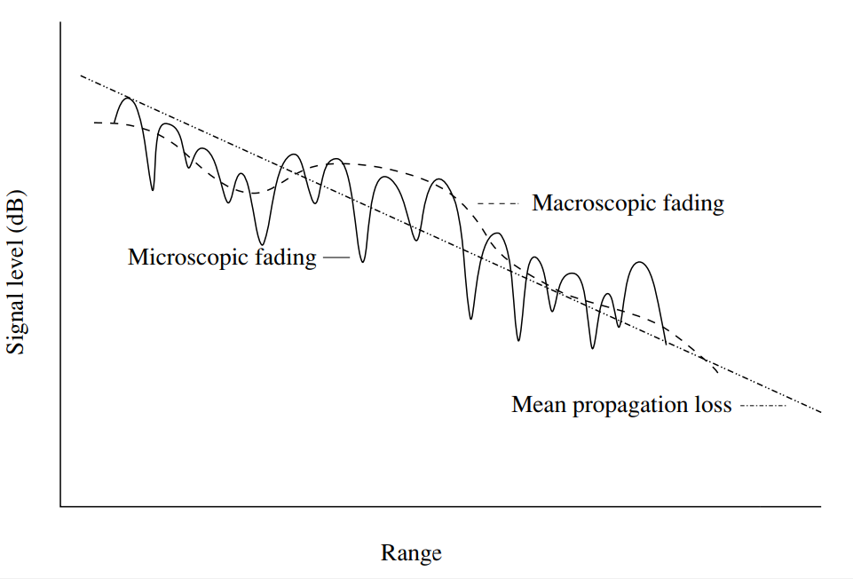 #
# > *Fig.1. Signal power fluctuation vs range in wireless channels. Mean propagation loss increases
# monotonically with range. Local deviations may occur due to macroscopic and microscopic fading \[1, p.14\].*
#
# So, firstly, the fading process can be classified based on appearence reasons:
#
# 
#
#
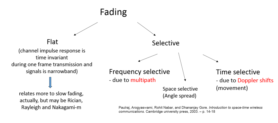
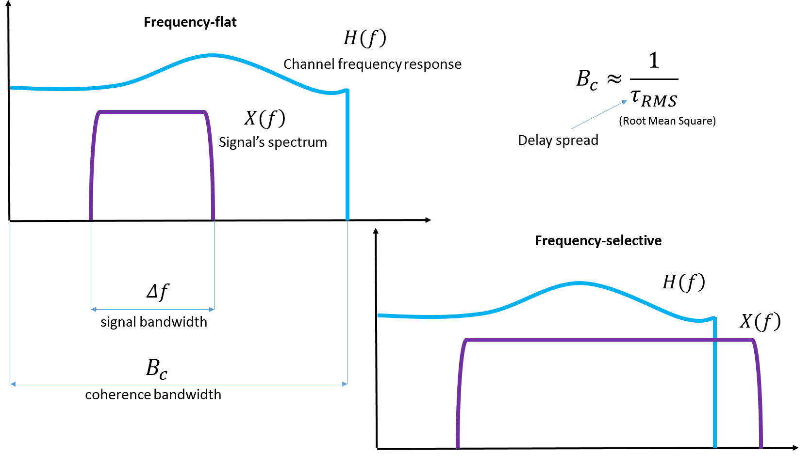
# However, fading can also be classified in dependence on channel characteristics: [coherence time](https://en.wikipedia.org/wiki/Coherence_time_(communications_systems)) of the channel $T_c$ and [coherence bandwidth](https://en.wikipedia.org/wiki/Coherence_bandwidth) $B_c$:
#
# 
#
# Only flat fading is considered during this research.
# ### What is the requirement to be frequency-flat?
#
# To obtain frequency-flat transmission the signal ***bit rate*** ($W = \Delta f$) should not exceed [coherence bandwidth](https://en.wikipedia.org/wiki/Coherence_bandwidth).
# 
#
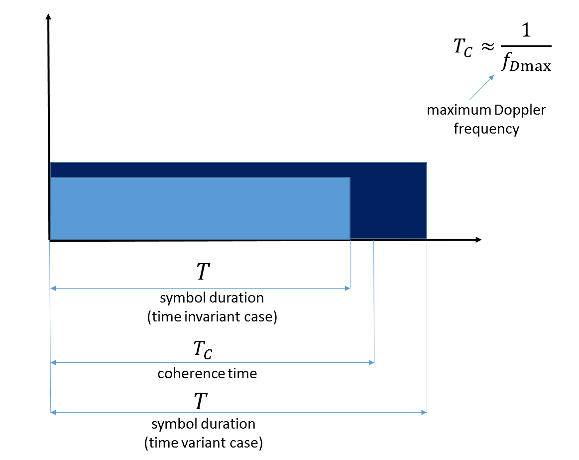
# ### What is the requirement to be time invarinat?
#
# To obtain frequency-flat transmission the signal ***duration*** ($T = \frac{1}{W}$) should not exceed [coherence time](https://en.wikipedia.org/wiki/https://en.wikipedia.org/wiki/Coherence_time).
#
#
# > *Fig.1. Signal power fluctuation vs range in wireless channels. Mean propagation loss increases
# monotonically with range. Local deviations may occur due to macroscopic and microscopic fading \[1, p.14\].*
#
# So, firstly, the fading process can be classified based on appearence reasons:
#
# 
#
#
# However, fading can also be classified in dependence on channel characteristics: [coherence time](https://en.wikipedia.org/wiki/Coherence_time_(communications_systems)) of the channel $T_c$ and [coherence bandwidth](https://en.wikipedia.org/wiki/Coherence_bandwidth) $B_c$:
#
# 
#
# Only flat fading is considered during this research.
# ### What is the requirement to be frequency-flat?
#
# To obtain frequency-flat transmission the signal ***bit rate*** ($W = \Delta f$) should not exceed [coherence bandwidth](https://en.wikipedia.org/wiki/Coherence_bandwidth).
# 
#
# ### What is the requirement to be time invarinat?
#
# To obtain frequency-flat transmission the signal ***duration*** ($T = \frac{1}{W}$) should not exceed [coherence time](https://en.wikipedia.org/wiki/https://en.wikipedia.org/wiki/Coherence_time).
#  #
# ### Sugested literature
# * Goldsmith A. Wireless communications. – Cambridge university press, 2005. – p. 88-92
#
# * Kanatas A. G., Panagopoulos A. D. (ed.). Radio Wave Propagation and Channel Modeling for Earth–Space Systems. – CRC Press, 2016. - p. 107
# ## Generalized Channel model
# Rician flat uncorrelated fading channel can be estimated based on described in [\[2\]](https://pdfs.semanticscholar.org/0fdd/65ed5a4e90f2ee44a1a0a8caa3f7021ce9f9.pdf) math model (MIMO system with linear arrays):
#
# $$
# \mathbf{H} = \sqrt{\frac{K}{K+1}}\mathbf{H_{LoS}} + \sqrt{\frac{1} {K+1}}\mathbf{H_{NLoS}} \qquad (1)
# $$
#
# where $\mathbf{H}$ is the channel matrix, $K$ is the Rician factor, $\mathbf{H_{LoS}}$ is the Line-of-Sight component and $\mathbf{H_{NLoS}}$ is the Non-Line-of-Sight component.
#
#
# ## Line-of-Sight component
# The term $\sqrt{\frac{K}{K+1}}\mathbf{H}_{LoS} = E\{H\}$ represents the mean component of the channel matrix and can be modeled according to geometrical approach:
#
# $$\mathbf{H}_{LoS} = \mathbf{a}_R(\theta_R)\mathbf{a}_T(\theta_T)^H \qquad (2)$$
#
# where $\mathbf{a}_R(\theta_R)$ and $\mathbf{a}_T(\theta_T)$ are the receive array and transmitt array responses, and $\theta_R$ and $\theta_T$ are the angls of arrival and departure.
# Array response can be expressed as:
# $$ \mathbf{a} = \left[1, e^{j2\pi d cos(\theta)},..., e^{j2\pi d(N-1) cos(\theta)} \right] \qquad (3)$$
#
# where $d$ is the antenna spacing in wavelenghts, $N$ is the number of the array elements.
#
#
# ### Sugested literature
# * Goldsmith A. Wireless communications. – Cambridge university press, 2005. – p. 88-92
#
# * Kanatas A. G., Panagopoulos A. D. (ed.). Radio Wave Propagation and Channel Modeling for Earth–Space Systems. – CRC Press, 2016. - p. 107
# ## Generalized Channel model
# Rician flat uncorrelated fading channel can be estimated based on described in [\[2\]](https://pdfs.semanticscholar.org/0fdd/65ed5a4e90f2ee44a1a0a8caa3f7021ce9f9.pdf) math model (MIMO system with linear arrays):
#
# $$
# \mathbf{H} = \sqrt{\frac{K}{K+1}}\mathbf{H_{LoS}} + \sqrt{\frac{1} {K+1}}\mathbf{H_{NLoS}} \qquad (1)
# $$
#
# where $\mathbf{H}$ is the channel matrix, $K$ is the Rician factor, $\mathbf{H_{LoS}}$ is the Line-of-Sight component and $\mathbf{H_{NLoS}}$ is the Non-Line-of-Sight component.
#
#
# ## Line-of-Sight component
# The term $\sqrt{\frac{K}{K+1}}\mathbf{H}_{LoS} = E\{H\}$ represents the mean component of the channel matrix and can be modeled according to geometrical approach:
#
# $$\mathbf{H}_{LoS} = \mathbf{a}_R(\theta_R)\mathbf{a}_T(\theta_T)^H \qquad (2)$$
#
# where $\mathbf{a}_R(\theta_R)$ and $\mathbf{a}_T(\theta_T)$ are the receive array and transmitt array responses, and $\theta_R$ and $\theta_T$ are the angls of arrival and departure.
# Array response can be expressed as:
# $$ \mathbf{a} = \left[1, e^{j2\pi d cos(\theta)},..., e^{j2\pi d(N-1) cos(\theta)} \right] \qquad (3)$$
#
# where $d$ is the antenna spacing in wavelenghts, $N$ is the number of the array elements.
# 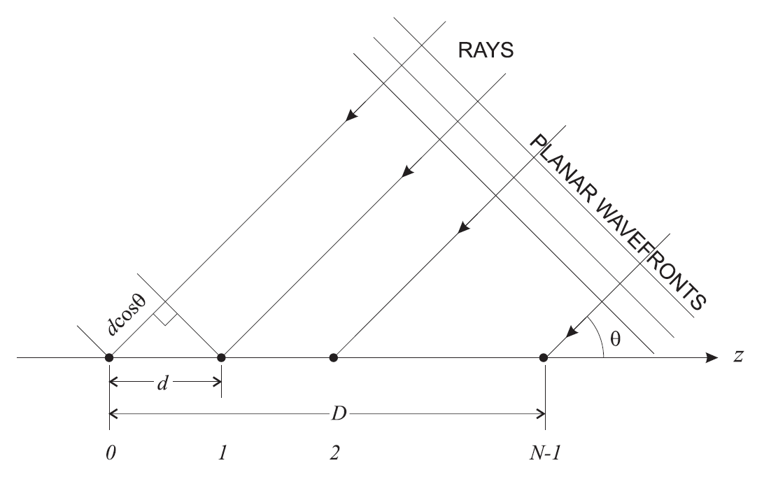 #
# > *Fig. 2. [Linear array geometry](http://www.waves.toronto.edu/prof/svhum/ece422/notes/15-arrays2.pdf).*
#
#
# ### Task:
# What is the squared Frobenius norm of the LoS component?
#
# ## Non-LoS componenet
# NLoS component can be classicaly modeled as the matrix of **IID** (independent identicaly distributed) **ZMCSCG** (zero mean
# circularly symmetric complex Gaussian) random values (amplitudes) [1, p. 39]:
#
# $$ Z = X + jY \qquad (4)$$
#
# where $X \sim \mathcal{N}(0,\,\sigma^2)$ and $Y \sim \mathcal{N}(0,\,\sigma^2)$. Frequently, the model with normalized average power is used, such that:
#
# $$ var\{Z\} = E\{\left|Z\right|^2\} = 1 \qquad (5)$$
#
# Hence, $Z \sim \mathcal{N}(0,\,1)$. Moreover, for independent distortions of both in-phase and quadrature signal components envolope can be described as the Rayleigh process \[3, p.78\]:
#
# $$ Z = \sqrt{\hat{X}^2 + \hat{Y}^2} \qquad (6)$$
#
# where $\hat{X} \sim \mathcal{N}(0,\,\sigma^2)$ and $\hat{Y} \sim \mathcal{N}(0,\,\sigma^2)$.
#
# 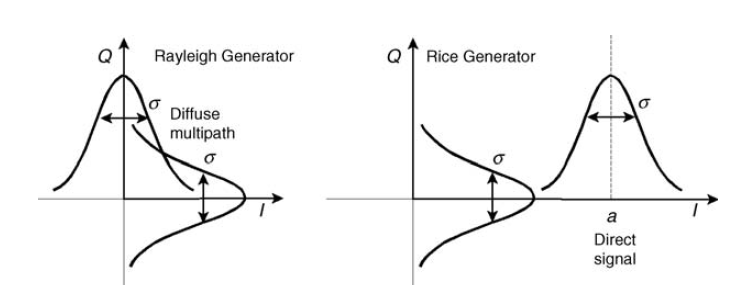
# > *Fig. 3. Gaussian generators in quadrature for simulating Rayleigh and Rice fades [\[4, p.125\]](https://s3.amazonaws.com/academia.edu.documents/45934974/Modelling.the.Wireless.Propagation.Channel.A.simulation.approach.with.Matlab.pdf?AWSAccessKeyId=AKIAIWOWYYGZ2Y53UL3A&Expires=1542970346&Signature=IkBGDMI6ref5QrEwFz2RG6Ns7vI%3D&response-content-disposition=inline%3B%20filename%3DModelling.the.Wireless.Propagation.Chann.pdf)*
#
# Actually, these phenomena mean Rayleigh fading (spatialy white) channel with scale factor $ \sigma = \frac{1}{\sqrt{2}} $ which can be modeled as [\[4, p.125\]](https://s3.amazonaws.com/academia.edu.documents/45934974/Modelling.the.Wireless.Propagation.Channel.A.simulation.approach.with.Matlab.pdf?AWSAccessKeyId=AKIAIWOWYYGZ2Y53UL3A&Expires=1542970346&Signature=IkBGDMI6ref5QrEwFz2RG6Ns7vI%3D&response-content-disposition=inline%3B%20filename%3DModelling.the.Wireless.Propagation.Chann.pdf):
#
# $$ \mathbf{H}_{NLoS} = \sqrt{\frac{1}{2}}\left(G_1+jG_2\right) \qquad (7)$$
#
# where $\mathbf{G}_1 \sim \mathcal{N}(0,\,1)$ and $\mathbf{G}_2 \sim \mathcal{N}(0,\,1)$ are consisting of the normaly distributed values matrices.
# ## Single antenna simplification
# Channel model with simplification to **SISO** case will have the following form:
#
# $$
# h = \sqrt{\frac{K}{K+1}} + \sqrt{\frac{1}{2(K+1)}}\left(G_1+jG_2\right) \qquad (8)
# $$
#
# And can be described via the following figure:
#
# 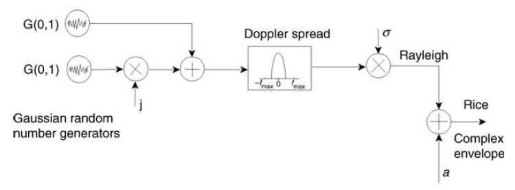
# > *Fig.4. Schematic diagram of the Rayleigh/Rice simulator (narrowband channel) [\[4, p.127\]](https://s3.amazonaws.com/academia.edu.documents/45934974/Modelling.the.Wireless.Propagation.Channel.A.simulation.approach.with.Matlab.pdf?AWSAccessKeyId=AKIAIWOWYYGZ2Y53UL3A&Expires=1542970346&Signature=IkBGDMI6ref5QrEwFz2RG6Ns7vI%3D&response-content-disposition=inline%3B%20filename%3DModelling.the.Wireless.Propagation.Chann.pdf)*.
#
# where $\sigma = \sqrt{\frac{1}{2(K+1)}}$ is Rician scale parameter and $a = \sqrt{\frac{K}{K+1}} $ is the Rician noncentrality parameter.
#
# > **NOTE THAT**:
# >
# >We are considering the flat fading channel and therefore assume Doppler spreadimpact as neglectable.
# > **NOTE THAT**:
# >
# > Classical Additive White Gaussian Noise \(AWGN\) model was selected (complex signal case) for the modeling of an additive noise. Nice explanation can be found via the [following link](https://www.gaussianwaves.com/2015/06/how-to-generate-awgn-noise-in-matlaboctave-without-using-in-built-awgn-function/).
#
# > **NOTE THAT**:
# >
# >The method how to estimate ergodic capacity usung the channel model can be obtained via the [following link](https://www.gaussianwaves.com/2014/09/ergodic-capacity-of-a-siso-system-over-a-rayleigh-fading-channel-simulation-in-matlab/).
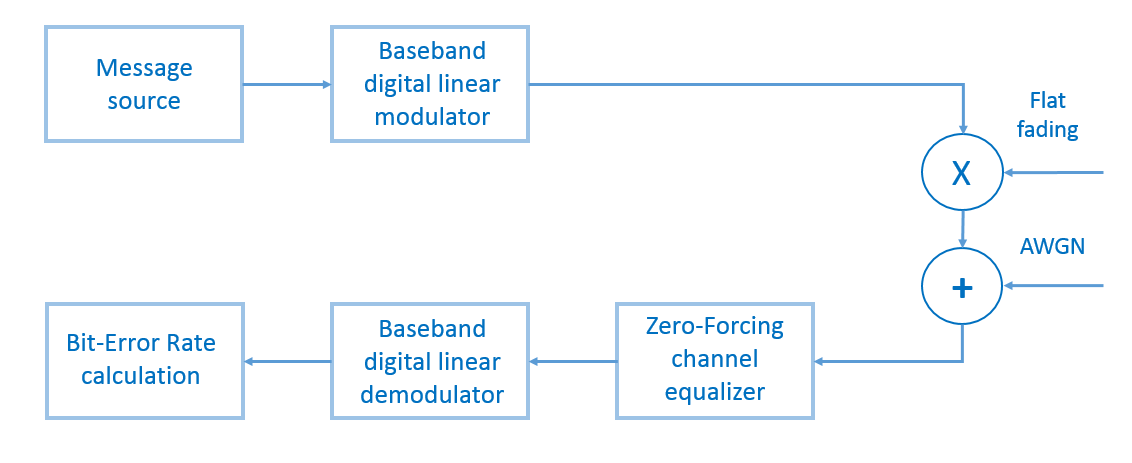
# ## Model verification
#
# For verification of the proposal model we model random binary message \(length of the message equals to 100000 bits\), modulate it by M-PSK / M-QAM (Gray mapping rule), multiply elementwise with fading process, add white gaussian noise, equalize by Zero-Forcing method, demodulate and calculate BER. The number of trials is equal to 100.
#
#
#
# > *Fig. 2. [Linear array geometry](http://www.waves.toronto.edu/prof/svhum/ece422/notes/15-arrays2.pdf).*
#
#
# ### Task:
# What is the squared Frobenius norm of the LoS component?
#
# ## Non-LoS componenet
# NLoS component can be classicaly modeled as the matrix of **IID** (independent identicaly distributed) **ZMCSCG** (zero mean
# circularly symmetric complex Gaussian) random values (amplitudes) [1, p. 39]:
#
# $$ Z = X + jY \qquad (4)$$
#
# where $X \sim \mathcal{N}(0,\,\sigma^2)$ and $Y \sim \mathcal{N}(0,\,\sigma^2)$. Frequently, the model with normalized average power is used, such that:
#
# $$ var\{Z\} = E\{\left|Z\right|^2\} = 1 \qquad (5)$$
#
# Hence, $Z \sim \mathcal{N}(0,\,1)$. Moreover, for independent distortions of both in-phase and quadrature signal components envolope can be described as the Rayleigh process \[3, p.78\]:
#
# $$ Z = \sqrt{\hat{X}^2 + \hat{Y}^2} \qquad (6)$$
#
# where $\hat{X} \sim \mathcal{N}(0,\,\sigma^2)$ and $\hat{Y} \sim \mathcal{N}(0,\,\sigma^2)$.
#
# 
# > *Fig. 3. Gaussian generators in quadrature for simulating Rayleigh and Rice fades [\[4, p.125\]](https://s3.amazonaws.com/academia.edu.documents/45934974/Modelling.the.Wireless.Propagation.Channel.A.simulation.approach.with.Matlab.pdf?AWSAccessKeyId=AKIAIWOWYYGZ2Y53UL3A&Expires=1542970346&Signature=IkBGDMI6ref5QrEwFz2RG6Ns7vI%3D&response-content-disposition=inline%3B%20filename%3DModelling.the.Wireless.Propagation.Chann.pdf)*
#
# Actually, these phenomena mean Rayleigh fading (spatialy white) channel with scale factor $ \sigma = \frac{1}{\sqrt{2}} $ which can be modeled as [\[4, p.125\]](https://s3.amazonaws.com/academia.edu.documents/45934974/Modelling.the.Wireless.Propagation.Channel.A.simulation.approach.with.Matlab.pdf?AWSAccessKeyId=AKIAIWOWYYGZ2Y53UL3A&Expires=1542970346&Signature=IkBGDMI6ref5QrEwFz2RG6Ns7vI%3D&response-content-disposition=inline%3B%20filename%3DModelling.the.Wireless.Propagation.Chann.pdf):
#
# $$ \mathbf{H}_{NLoS} = \sqrt{\frac{1}{2}}\left(G_1+jG_2\right) \qquad (7)$$
#
# where $\mathbf{G}_1 \sim \mathcal{N}(0,\,1)$ and $\mathbf{G}_2 \sim \mathcal{N}(0,\,1)$ are consisting of the normaly distributed values matrices.
# ## Single antenna simplification
# Channel model with simplification to **SISO** case will have the following form:
#
# $$
# h = \sqrt{\frac{K}{K+1}} + \sqrt{\frac{1}{2(K+1)}}\left(G_1+jG_2\right) \qquad (8)
# $$
#
# And can be described via the following figure:
#
# 
# > *Fig.4. Schematic diagram of the Rayleigh/Rice simulator (narrowband channel) [\[4, p.127\]](https://s3.amazonaws.com/academia.edu.documents/45934974/Modelling.the.Wireless.Propagation.Channel.A.simulation.approach.with.Matlab.pdf?AWSAccessKeyId=AKIAIWOWYYGZ2Y53UL3A&Expires=1542970346&Signature=IkBGDMI6ref5QrEwFz2RG6Ns7vI%3D&response-content-disposition=inline%3B%20filename%3DModelling.the.Wireless.Propagation.Chann.pdf)*.
#
# where $\sigma = \sqrt{\frac{1}{2(K+1)}}$ is Rician scale parameter and $a = \sqrt{\frac{K}{K+1}} $ is the Rician noncentrality parameter.
#
# > **NOTE THAT**:
# >
# >We are considering the flat fading channel and therefore assume Doppler spreadimpact as neglectable.
# > **NOTE THAT**:
# >
# > Classical Additive White Gaussian Noise \(AWGN\) model was selected (complex signal case) for the modeling of an additive noise. Nice explanation can be found via the [following link](https://www.gaussianwaves.com/2015/06/how-to-generate-awgn-noise-in-matlaboctave-without-using-in-built-awgn-function/).
#
# > **NOTE THAT**:
# >
# >The method how to estimate ergodic capacity usung the channel model can be obtained via the [following link](https://www.gaussianwaves.com/2014/09/ergodic-capacity-of-a-siso-system-over-a-rayleigh-fading-channel-simulation-in-matlab/).
# ## Model verification
#
# For verification of the proposal model we model random binary message \(length of the message equals to 100000 bits\), modulate it by M-PSK / M-QAM (Gray mapping rule), multiply elementwise with fading process, add white gaussian noise, equalize by Zero-Forcing method, demodulate and calculate BER. The number of trials is equal to 100.
#
#  # > **Simulation script**:
# >
# >Vladimir Fadeev (2019). M-PSK and M-QAM over Rician flat fading channel (https://www.mathworks.com/matlabcentral/fileexchange/70559-m-psk-and-m-qam-over-rician-flat-fading-channel), MATLAB Central File Exchange. Retrieved October 7, 2019.
# 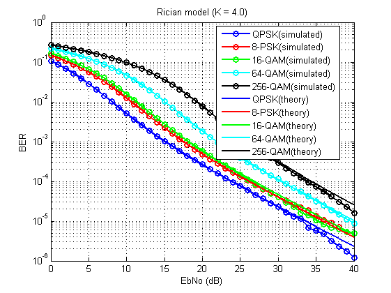
# >*Fig. 5. Bit error ratio performance of described ways of the modeling (K = 4.0).*
#
# 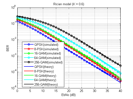
# >*Fig. 6. Bit error ratio performance of described ways of the modeling (K = 0.6).*
#
# As we can see in figures 5 and 6 BER performance of the proposal approaches completely matched with theoretical \(**berfading\(\) function in MatLab**\) results.
#
# # References
#
# 1. Paulraj, Arogyaswami, Rohit Nabar, and Dhananjay Gore. Introduction to space-time wireless communications. Cambridge university press, 2003.
#
# 2. Farrokhi, Farrokh R., et al. "Spectral efficiency of FDMA/TDMA wireless systems with transmit and receive antenna arrays." IEEE transactions on wireless communications 1.4 (2002): 591-599.
#
# 3. Goldsmith A. Wireless communications. – Cambridge university press, 2005.
#
# 4. Fontæn, Fernando Pærez, and Perfecto Mariæo Espiæeira. Modelling the wireless propagation channel: a simulation approach with Matlab. Vol. 5. John Wiley & Sons, 2008.
#
#
# ## Task solution
#
#
# $$ ||H_{LoS}||^2_F = \sum^{M_R}_{i=1}\sum^{M_T}_{j=1}|h^{(LoS)}_{ij}|^2 $$
#
# What is the $h^{(LoS)}_{ij}$? It is the **complex exponent** (e.g. $e^{j\phi}$) anyway. Each complex exponent can be represented as the sum of the *cos* and *sin* components:
#
# $$ e^{j\phi} = cos\phi + jsin\phi $$
#
# The squared absolute value of the complex value $z = x +jy$:
#
# $$ |z|^2 = x^2 + y^2 $$
#
# Hence:
#
# $$ |e^{j\phi}|^2 = cos^2\phi + sin^2\phi = 1 $$
#
# And finally:
#
# $$ ||H_{LoS}||^2_F = M_RM_T $$
#
# > **Simulation script**:
# >
# >Vladimir Fadeev (2019). M-PSK and M-QAM over Rician flat fading channel (https://www.mathworks.com/matlabcentral/fileexchange/70559-m-psk-and-m-qam-over-rician-flat-fading-channel), MATLAB Central File Exchange. Retrieved October 7, 2019.
# 
# >*Fig. 5. Bit error ratio performance of described ways of the modeling (K = 4.0).*
#
# 
# >*Fig. 6. Bit error ratio performance of described ways of the modeling (K = 0.6).*
#
# As we can see in figures 5 and 6 BER performance of the proposal approaches completely matched with theoretical \(**berfading\(\) function in MatLab**\) results.
#
# # References
#
# 1. Paulraj, Arogyaswami, Rohit Nabar, and Dhananjay Gore. Introduction to space-time wireless communications. Cambridge university press, 2003.
#
# 2. Farrokhi, Farrokh R., et al. "Spectral efficiency of FDMA/TDMA wireless systems with transmit and receive antenna arrays." IEEE transactions on wireless communications 1.4 (2002): 591-599.
#
# 3. Goldsmith A. Wireless communications. – Cambridge university press, 2005.
#
# 4. Fontæn, Fernando Pærez, and Perfecto Mariæo Espiæeira. Modelling the wireless propagation channel: a simulation approach with Matlab. Vol. 5. John Wiley & Sons, 2008.
#
#
# ## Task solution
#
#
# $$ ||H_{LoS}||^2_F = \sum^{M_R}_{i=1}\sum^{M_T}_{j=1}|h^{(LoS)}_{ij}|^2 $$
#
# What is the $h^{(LoS)}_{ij}$? It is the **complex exponent** (e.g. $e^{j\phi}$) anyway. Each complex exponent can be represented as the sum of the *cos* and *sin* components:
#
# $$ e^{j\phi} = cos\phi + jsin\phi $$
#
# The squared absolute value of the complex value $z = x +jy$:
#
# $$ |z|^2 = x^2 + y^2 $$
#
# Hence:
#
# $$ |e^{j\phi}|^2 = cos^2\phi + sin^2\phi = 1 $$
#
# And finally:
#
# $$ ||H_{LoS}||^2_F = M_RM_T $$
#