#!/usr/bin/env python
# coding: utf-8
# # Introducing Pandas Objects
#
# Pandas objects can be thought of as enhanced versions of NumPy structured arrays in which the rows and columns are identified with labels rather than simple integer indices.
#
# Let's introduce these three fundamental Pandas data structures: the ``Series``, ``DataFrame``, and ``Index``.
# In[14]:
import numpy as np
import pandas as pd
# ## The Pandas Series Object
#
# A Pandas ``Series`` is a one-dimensional array of indexed data:
# In[15]:
data = pd.Series([0.25, 0.5, 0.75, 1.0])
data
# ``Series`` objects wrap both a sequence of values and a sequence of indices, which we can access with the ``values`` and ``index`` attributes.
#
# The ``values`` are simply a familiar NumPy array:
# In[16]:
data.values
# In[17]:
type(_)
# The ``index`` is an array-like object of type ``pd.Index``:
# In[18]:
data.index
# In[19]:
print(pd.RangeIndex.__doc__)
# Like with a NumPy array, data can be accessed by the associated index via the familiar Python square-bracket notation:
# In[20]:
data[1]
# In[21]:
data[1:3]
# In[22]:
type(_)
# ### ``Series`` as generalized NumPy array
#
# It may look like the ``Series`` object is basically interchangeable with a one-dimensional NumPy array.
# The essential difference is the presence of the index: while the Numpy Array has an *implicitly defined* integer index used to access the values, the Pandas ``Series`` has an *explicitly defined* index associated with the values.
#
# In[23]:
data = pd.Series([0.25, 0.5, 0.75, 1.0], index=['a', 'b', 'c', 'd'])
data
# In[24]:
data['b'] # item access works as expected
# We can even use non-contiguous or non-sequential indices:
# In[25]:
data = pd.Series([0.25, 0.5, 0.75, 1.0], index=[2, 5, 3, 7])
data
# In[11]:
data[5]
# ### Series as specialized dictionary
#
# You can think of a Pandas ``Series`` a bit like a specialization of a Python dictionary.
# A dictionary is a structure that maps arbitrary keys to a set of arbitrary values, and a ``Series`` is a structure which maps typed keys to a set of typed values:
# In[27]:
population_dict = {'California': 38332521,
'Texas': 26448193,
'New York': 19651127,
'Florida': 19552860,
'Illinois': 12882135}
population = pd.Series(population_dict)
population
# In[28]:
type(_)
# In[29]:
population.index
# In[30]:
population['California'] # typical dictionary-style item access
# In[31]:
population['California':'Illinois'] # array-like slicing
# ## The Pandas DataFrame Object
#
# The next fundamental structure in Pandas is the ``DataFrame`` which can be thought of either as a generalization of a NumPy array, or as a specialization of a Python dictionary.
# ### DataFrame as a generalized NumPy array
# If a ``Series`` is an analog of a one-dimensional array with flexible indices, a ``DataFrame`` is an analog of a two-dimensional array with both flexible row indices and flexible column names.
#
# You can think of a ``DataFrame`` as a sequence of _aligned_ ``Series`` objects.
# Here, by _aligned_ we mean that they share the same index:
# In[32]:
area_dict = {'California': 423967, 'Texas': 695662, 'New York': 141297,
'Florida': 170312, 'Illinois': 149995}
area = pd.Series(area_dict)
area
# In[36]:
states = pd.DataFrame({'population': population, 'area': area})
states
# In[37]:
type(_)
# In[38]:
states.index
# Additionally, the ``DataFrame`` has a ``columns`` attribute, which is an ``Index`` object holding the column labels:
# In[39]:
states.columns
# In[40]:
type(_)
# Thus the ``DataFrame`` can be thought of as a generalization of a two-dimensional NumPy array, where both the rows and columns have a generalized index for accessing the data.
# ### DataFrame as specialized dictionary
#
# Similarly, we can also think of a ``DataFrame`` as a specialization of a dictionary.
#
# Where a dictionary maps a key to a value, a ``DataFrame`` maps a column name to a ``Series`` of column data:
# In[41]:
states['area'] # "feature"
# ### Constructing DataFrame objects
# #### From a single Series object
#
# A ``DataFrame`` is a collection of ``Series`` objects, and a single-column ``DataFrame`` can be constructed from a single ``Series``:
#
# In[42]:
pd.DataFrame(population, columns=['population'])
# #### From a list of dicts
#
#
# In[48]:
data = [{'a': i, 'b': 2 * i} for i in range(3)]
data
# In[49]:
pd.DataFrame(data)
# In[23]:
pd.DataFrame([{'a': 1, 'b': 2}, {'b': 3, 'c': 4}]) # Pandas will fill missing keys with ``NaN``
# #### From a two-dimensional NumPy array
#
# Given a two-dimensional array of data, we can create a ``DataFrame`` with any specified column and index names:
# In[50]:
np.random.rand(3, 2)
# In[51]:
pd.DataFrame(np.random.rand(3, 2),
columns=['foo', 'bar'],
index=['a', 'b', 'c'])
# #### From a NumPy structured array
# In[52]:
A = np.zeros(3, dtype=[('A', 'i8'), ('B', 'f8')])
A
# In[53]:
pd.DataFrame(A)
# ## The Pandas Index Object
#
# This ``Index`` object is an interesting structure in itself, and it can be thought of either as an *immutable array* or as an *ordered set* (technically a multi-set, as ``Index`` objects may contain repeated values).
#
# In[55]:
ind = pd.Index([2, 3, 5, 7, 11])
ind
# ### Index as immutable array
#
# The ``Index`` in many ways operates like an array.
#
# In[56]:
ind[1]
# In[58]:
ind[::2]
# ``Index`` objects also have many of the attributes familiar from NumPy arrays:
# In[59]:
ind.size, ind.shape, ind.ndim, ind.dtype,
# One difference is that indices are immutable–that is, they cannot be modified via the normal means:
# In[60]:
ind[1] = 0
# ### Index as ordered set
#
# The ``Index`` object follows many of the conventions used by Python's built-in ``set`` data structure, so that unions, intersections, differences, and other combinations can be computed in a familiar way:
# In[61]:
indA = pd.Index([1, 3, 5, 7, 9])
indB = pd.Index([2, 3, 5, 7, 11])
# In[62]:
indA.intersection(indB) # intersection
# In[39]:
indA.union(indB) # union
# In[40]:
indA.symmetric_difference(indB) # symmetric difference
# # Data Indexing and Selection
#
# To modify values in NumPy arrays we use indexing (e.g., ``arr[2, 1]``), slicing (e.g., ``arr[:, 1:5]``), masking (e.g., ``arr[arr > 0]``), fancy indexing (e.g., ``arr[0, [1, 5]]``), and combinations thereof (e.g., ``arr[:, [1, 5]]``).
#
# Here we'll look at similar means of accessing and modifying values in Pandas ``Series`` and ``DataFrame`` objects.
# If you have used the NumPy patterns, the corresponding patterns in Pandas will feel very familiar, though there are a few quirks to be aware of.
#
# ## Data Selection in Series
#
# A ``Series`` object acts in many ways like a one-dimensional NumPy array, and in many ways like a standard Python dictionary.
# ### Series as dictionary
#
# Like a dictionary, the ``Series`` object provides a mapping from a collection of keys to a collection of values:
# In[63]:
data = pd.Series([0.25, 0.5, 0.75, 1.0], index=['a', 'b', 'c', 'd'])
data
# In[64]:
data['b'] # mnemonic indexing
# In[65]:
'a' in data # dictionary-like Python expressions...
# In[67]:
data.keys() # ...and methods.
# In[68]:
list(data.items())
# ``Series`` objects can even be modified with a dictionary-like syntax:
# In[69]:
data['e'] = 1.25
data
# This easy mutability of the objects is a convenient feature: under the hood, Pandas is making decisions about memory layout and data copying that might need to take place.
# ### Series as one-dimensional array
#
# A ``Series`` builds on this dictionary-like interface and provides array-style item selection via the same basic mechanisms as NumPy arrays – that is, *slices*, *masking*, and *fancy indexing*:
# In[47]:
data['a':'c'] # slicing by explicit index
# In[48]:
data[0:2] # slicing by implicit integer index
# In[49]:
data[(data > 0.3) & (data < 0.8)] # masking
# because
# In[70]:
(data > 0.3) & (data < 0.8)
# In[71]:
type(_)
# In[50]:
data[['a', 'e']] # fancy indexing
# Notice that when slicing with an explicit index (i.e., ``data['a':'c']``), the final index is *included* in the slice, while when slicing with an implicit index (i.e., ``data[0:2]``), the final index is *excluded* from the slice.
# ### Indexers: loc, iloc, and ix
#
# If your ``Series`` has an explicit integer index, an indexing operation such as ``data[1]`` will use the explicit indices, while a slicing operation like ``data[1:3]`` will use the implicit Python-style index.
# In[72]:
data = pd.Series(['a', 'b', 'c'], index=[1, 3, 5])
data
# In[73]:
data[1] # explicit index when indexing
# In[74]:
data[1:3] # implicit index when slicing
# Because of this potential confusion in the case of integer indexes, Pandas provides some special *indexer* attributes that explicitly expose certain indexing schemes.
#
# These are not functional methods, but attributes that expose a particular slicing interface to the data in the ``Series``.
# First, the ``loc`` attribute allows indexing and slicing that always references the explicit index:
# In[75]:
data.loc[1]
# In[76]:
data.loc[1:3]
# The ``iloc`` attribute allows indexing and slicing that always references the implicit Python-style index:
# In[77]:
data.iloc[1:3]
# A third indexing attribute, ``ix``, is a hybrid of the two, and for ``Series`` objects is equivalent to standard ``[]``-based indexing.
#
# The purpose of the ``ix`` indexer will become more apparent in the context of ``DataFrame`` objects.
# ## Data Selection in DataFrame
#
# Recall that a ``DataFrame`` acts in many ways like a two-dimensional or structured array, and in other ways like a dictionary of ``Series`` structures sharing the same index.
# In[78]:
area = pd.Series({'California': 423967, 'Texas': 695662,
'New York': 141297, 'Florida': 170312,
'Illinois': 149995})
pop = pd.Series({'California': 38332521, 'Texas': 26448193,
'New York': 19651127, 'Florida': 19552860,
'Illinois': 12882135})
# In[79]:
data = pd.DataFrame({'area':area, 'pop':pop})
data
# In[80]:
data['area'] # columns can be accessed via dict-style indexing
# In[81]:
data.area # alternatively, use attribute-style access with column names
# this dictionary-style syntax can also be used to modify the object, in this case adding a new column:
# In[82]:
data['density'] = data['pop'] / data['area']
data
# ### DataFrame as two-dimensional array
#
# ``DataFrame`` can also be viewed as an enhanced two-dimensional array:
# In[83]:
data.values # examine the raw underlying data array
# In[87]:
data.values.T
# In[88]:
type(_)
# In[89]:
data.T # transpose the full DataFrame object
# In[90]:
type(_)
# In[91]:
data.values[0] # passing a single index to an array accesses a row
# In[92]:
data['area'] # assing a single "index" to access a column
# Using the ``iloc`` indexer, we can index the underlying array as if it is a simple NumPy array (using the implicit Python-style index)
# In[93]:
data.iloc[:3, :2]
# Similarly, using the ``loc`` indexer we can index the underlying data in an array-like style but using the explicit index and column names:
# In[67]:
data.loc[:'Illinois', :'pop']
# Any of the familiar NumPy-style data access patterns can be used within these indexers.
# In[68]:
data.loc[data.density > 100, ['pop', 'density']]
# Any of these indexing conventions may also be used to set or modify values; this is done in the standard way that you might be accustomed to from working with NumPy:
# In[69]:
data.iloc[0, 2] = 90
data
# ### Additional indexing conventions
# In[70]:
data['Florida':'Illinois'] # *slicing* refers to rows
# In[71]:
data[data.density > 100] # direct masking operations are also interpreted row-wise
# # Operating on Data in Pandas
#
# One of the essential pieces of NumPy is the ability to perform quick element-wise operations, both with basic arithmetic (addition, subtraction, multiplication, etc.) and with more sophisticated operations (trigonometric functions, exponential and logarithmic functions, etc.).
#
# Pandas inherits much of this functionality from NumPy.
#
# Pandas includes a couple useful twists, however: for unary operations like negation and trigonometric functions, these ufuncs will *preserve index and column labels* in the output, and for binary operations such as addition and multiplication, Pandas will automatically *align indices* when passing the objects to the ufunc.
# ## Ufuncs: Index Preservation
#
# Because Pandas is designed to work with NumPy, any NumPy ufunc will work on Pandas ``Series`` and ``DataFrame`` objects:
# In[94]:
rng = np.random.RandomState(42)
ser = pd.Series(rng.randint(0, 10, 4))
ser
# In[96]:
rng.randint(0, 10, (3, 4))
# In[97]:
df = pd.DataFrame(rng.randint(0, 10, (3, 4)), columns=['A', 'B', 'C', 'D'])
df
# If we apply a NumPy ufunc on either of these objects, the result will be another Pandas object *with the indices preserved:*
# In[100]:
np.exp(ser)
# In[101]:
type(_)
# In[102]:
np.sin(df * np.pi / 4) # a slightly more complex calculation
# In[103]:
type(_)
# ## UFuncs: Index Alignment
#
# For binary operations on two ``Series`` or ``DataFrame`` objects, Pandas will align indices in the process of performing the operation.
# ### Index alignment in Series
#
# Suppose we are combining two different data sources, and find only the top three US states by *area* and the top three US states by *population*:
# In[104]:
area = pd.Series({'Alaska': 1723337, 'Texas': 695662, 'California': 423967}, name='area')
population = pd.Series({'California': 38332521, 'Texas': 26448193, 'New York': 19651127}, name='population')
# In[106]:
population / area
# The resulting array contains the *union* of indices of the two input arrays, which could be determined using standard Python set arithmetic on these indices:
# In[107]:
area.index.union(population.index) # this does create a new index and doesn't modify in place.
# In[108]:
area.index
# Any item for which one or the other does not have an entry is marked with ``NaN``, or "Not a Number," which is how Pandas marks missing data
# .
# This index matching is implemented this way for any of Python's built-in arithmetic expressions; any missing values are filled in with NaN by default:
# In[109]:
A = pd.Series([2, 4, 6], index=[0, 1, 2])
B = pd.Series([1, 3, 5], index=[1, 2, 3])
A + B
# If using NaN values is not the desired behavior, the fill value can be modified using appropriate object methods in place of the operators:
# In[110]:
A.add(B, fill_value=0)
# ### Index alignment in DataFrame
#
# A similar type of alignment takes place for *both* columns and indices when performing operations on ``DataFrame``s:
# In[111]:
A = pd.DataFrame(rng.randint(0, 20, (2, 2)), columns=list('AB'))
A
# In[113]:
B = pd.DataFrame(rng.randint(0, 10, (3, 3)), columns=list('BAC'))
B
# In[114]:
A + B
# In[116]:
fill = A.stack().mean()
fill
# In[117]:
A.add(B, fill_value=fill)
# The following table lists Python operators and their equivalent Pandas object methods:
#
# | Python Operator | Pandas Method(s) |
# |-----------------|---------------------------------------|
# | ``+`` | ``add()`` |
# | ``-`` | ``sub()``, ``subtract()`` |
# | ``*`` | ``mul()``, ``multiply()`` |
# | ``/`` | ``truediv()``, ``div()``, ``divide()``|
# | ``//`` | ``floordiv()`` |
# | ``%`` | ``mod()`` |
# | ``**`` | ``pow()`` |
#
# ## Ufuncs: Operations Between DataFrame and Series
#
# When performing operations between a ``DataFrame`` and a ``Series``, the index and column alignment is similarly maintained.
# Operations between a ``DataFrame`` and a ``Series`` are similar to operations between a two-dimensional and one-dimensional NumPy array.
# In[87]:
A = rng.randint(10, size=(3, 4))
A
# In[89]:
type(A)
# In[88]:
A - A[0]
# According to NumPy's broadcasting rules , subtraction between a two-dimensional array and one of its rows is applied row-wise.
# In Pandas, the convention similarly operates row-wise by default:
# In[90]:
df = pd.DataFrame(A, columns=list('QRST'))
df - df.iloc[0]
# If you would instead like to operate column-wise you have to specify the ``axis`` keyword:
# In[91]:
df.subtract(df['R'], axis=0)
# # Handling Missing Data
#
# The difference between data found in many tutorials and data in the real world is that real-world data is rarely clean and homogeneous.
# In particular, many interesting datasets will have some amount of data missing.
#
# To make matters even more complicated, different data sources may indicate missing data in different ways.
# ## Trade-Offs in Missing Data Conventions
#
# To indicate the presence of missing data in a table or DataFrame we can use two strategies: using a *mask* that globally indicates missing values, or choosing a *sentinel value* that indicates a missing entry.
#
# In the masking approach, the mask might be an entirely separate Boolean array, or it may involve appropriation of one bit in the data representation to locally indicate the null status of a value.
#
# In the sentinel approach, the sentinel value could be some data-specific convention, such as indicating a missing integer value with -9999 or some rare bit pattern, or it could be a more global convention, such as indicating a missing floating-point value with NaN (Not a Number).
#
# None of these approaches is without trade-offs: use of a separate mask array requires allocation of an additional Boolean array. A sentinel value reduces the range of valid values that can be represented, and may require extra (often non-optimized) logic in CPU and GPU arithmetic.
# ## Missing Data in Pandas
#
# The way in which Pandas handles missing values is constrained by its reliance on the NumPy package, which does **not have** a built-in notion of NA values for non-floating-point data types.
#
# NumPy does have support for masked arrays – that is, arrays that have a separate Boolean mask array attached for marking data as "good" or "bad."
# Pandas could have derived from this, but the overhead in both storage, computation, and code maintenance makes that an unattractive choice.
#
# With these constraints in mind, Pandas chose to use sentinels for missing data, and further chose to use two already-existing Python null values: the special floating-point ``NaN`` value, and the Python ``None`` object.
# ### ``None``: Pythonic missing data
#
# The first sentinel value used by Pandas is ``None``, a Python singleton object that is often used for missing data in Python code.
#
# Because it is a Python object, ``None`` cannot be used in any arbitrary NumPy/Pandas array, but only in arrays with data type ``'object'`` (i.e., arrays of Python objects):
# In[118]:
vals1 = np.array([1, None, 3, 4])
vals1
# Any operations on the data will be done at the Python level, with much more overhead than the typically fast operations seen for arrays with native types:
# In[93]:
for dtype in ['object', 'int']:
print("dtype =", dtype)
get_ipython().run_line_magic('timeit', 'np.arange(1E6, dtype=dtype).sum()')
print()
# The use of Python objects in an array also means that if you perform aggregations like ``sum()`` or ``min()`` across an array with a ``None`` value, you will generally get an error:
# In[94]:
vals1.sum()
# ### ``NaN``: Missing numerical data
#
# The other missing data representation, ``NaN`` (acronym for *Not a Number*), is different; it is a special floating-point value recognized by all systems that use the standard IEEE floating-point representation:
# In[119]:
vals2 = np.array([1, np.nan, 3, 4])
vals2.dtype
# In[120]:
1 + np.nan, 0 * np.nan
# In[121]:
vals2.sum(), vals2.min(), vals2.max()
# NumPy does provide some special aggregations that will ignore these missing values:
# In[98]:
np.nansum(vals2), np.nanmin(vals2), np.nanmax(vals2)
# ### NaN and None in Pandas
#
# ``NaN`` and ``None`` both have their place, and Pandas is built to handle the two of them nearly interchangeably, converting between them where appropriate:
# In[99]:
pd.Series([1, np.nan, 2, None])
# The following table lists the upcasting conventions in Pandas when NA values are introduced:
#
# |Typeclass | Conversion When Storing NAs | NA Sentinel Value |
# |--------------|-----------------------------|------------------------|
# | ``floating`` | No change | ``np.nan`` |
# | ``object`` | No change | ``None`` or ``np.nan`` |
# | ``integer`` | Cast to ``float64`` | ``np.nan`` |
# | ``boolean`` | Cast to ``object`` | ``None`` or ``np.nan`` |
#
# Keep in mind that in Pandas, string data is always stored with an ``object`` dtype.
# ## Operating on Null Values
#
# As we have seen, Pandas treats ``None`` and ``NaN`` as essentially interchangeable for indicating missing or null values.
# To facilitate this convention, there are several useful methods for detecting, removing, and replacing null values in Pandas data structures.
# They are:
#
# - ``isnull()``: Generate a boolean mask indicating missing values
# - ``notnull()``: Opposite of ``isnull()``
# - ``dropna()``: Return a filtered version of the data
# - ``fillna()``: Return a copy of the data with missing values filled or imputed
# ### Detecting null values
# Pandas data structures have two useful methods for detecting null data: ``isnull()`` and ``notnull()``.
# Either one will return a Boolean mask over the data:
# In[122]:
data = pd.Series([1, np.nan, 'hello', None])
data.isnull()
# ### Dropping null values
#
# In addition to the masking used before, there are the convenience methods, ``dropna()``
# (which removes NA values) and ``fillna()`` (which fills in NA values):
# In[101]:
data.dropna()
# For a ``DataFrame``, there are more options:
# In[123]:
df = pd.DataFrame([[1, np.nan, 2],
[2, 3, 5],
[np.nan, 4, 6]])
df
# In[124]:
df.dropna() # drop all rows in which *any* null value is present
# In[104]:
df.dropna(axis='columns') # drop NA values from all columns containing a null value
# The default is ``how='any'``, such that any row or column (depending on the ``axis`` keyword) containing a null value will be dropped.
# In[105]:
df[3] = np.nan
df
# You can also specify ``how='all'``, which will only drop rows/columns that are *all* null values:
# In[106]:
df.dropna(axis='columns', how='all')
# The ``thresh`` parameter lets you specify a minimum number of non-null values for the row/column to be kept:
# In[107]:
df.dropna(axis='rows', thresh=3)
# ### Filling null values
#
# Sometimes rather than dropping NA values, you'd rather replace them with a valid value.
# This value might be a single number like zero, or it might be some sort of imputation or interpolation from the good values.
# You could do this in-place using the ``isnull()`` method as a mask, but because it is such a common operation Pandas provides the ``fillna()`` method, which returns a copy of the array with the null values replaced.
#
# In[108]:
data = pd.Series([1, np.nan, 2, None, 3], index=list('abcde'))
data
# In[109]:
data.fillna(0) # fill NA entries with a single value
# In[110]:
data.fillna(method='ffill') # specify a forward-fill to propagate the previous value forward
# In[111]:
data.fillna(method='bfill') # specify a back-fill to propagate the next values backward
# For ``DataFrame``s, the options are similar, but we can also specify an ``axis`` along which the fills take place:
# In[112]:
df
# In[113]:
df.fillna(method='ffill', axis=1)
# # Hierarchical Indexing
#
# Up to this point we've been focused primarily on one-dimensional and two-dimensional data, stored in Pandas ``Series`` and ``DataFrame`` objects, respectively.
# Often it is useful to go beyond this and store higher-dimensional data–that is, data indexed by more than one or two keys.
#
# A far more common pattern in practice is to make use of *hierarchical indexing* (also known as *multi-indexing*) to incorporate multiple index *levels* within a single index.
# In this way, higher-dimensional data can be compactly represented within the familiar one-dimensional ``Series`` and two-dimensional ``DataFrame`` objects.
#
# ## A Multiply Indexed Series
#
# Let's start by considering how we might represent two-dimensional data within a one-dimensional ``Series``.
# ### The bad way
#
# Suppose you would like to track data about states from two different years.
# Using the Pandas tools we've already covered, you might be tempted to simply use Python tuples as keys:
# In[125]:
index = [('California', 2000), ('California', 2010),
('New York', 2000), ('New York', 2010),
('Texas', 2000), ('Texas', 2010)]
populations = [33871648, 37253956,
18976457, 19378102,
20851820, 25145561]
pop = pd.Series(populations, index=index)
pop
# If you need to select all values from 2010, you'll need to do some messy (and potentially slow) munging to make it happen:
# In[115]:
pop[[i for i in pop.index if i[1] == 2010]]
# ### The Better Way: Pandas MultiIndex
#
# Our tuple-based indexing is essentially a rudimentary multi-index, and the Pandas ``MultiIndex`` type gives us the type of operations we wish to have:
# In[126]:
index = pd.MultiIndex.from_tuples(index)
index
# In[127]:
type(_)
# A ``MultiIndex`` contains multiple *levels* of indexing–in this case, the state names and the years, as well as multiple *labels* for each data point which encode these levels.
# If we re-index our series with this ``MultiIndex``, we see the hierarchical representation of the data:
# In[128]:
pop = pop.reindex(index)
pop
# Here the first two columns of the ``Series`` representation show the multiple index values, while the third column shows the data.
#
# Notice that some entries are missing in the first column: in this multi-index representation, any blank entry indicates the same value as the line above it.
# Now to access all data for which the second index is 2010, we can simply use the Pandas slicing notation:
# In[118]:
pop[:, 2010]
# The result is a singly indexed array with just the keys we're interested in.
# This syntax is much more convenient (and the operation is much more efficient!) than the home-spun tuple-based multi-indexing solution that we started with.
#
# ### MultiIndex as extra dimension
#
# We could have stored the same data using a simple ``DataFrame`` with index and column labels; in fact, Pandas is built with this equivalence in mind.
#
# The ``unstack()`` method will quickly convert a multiply indexed ``Series`` into a conventionally indexed ``DataFrame``:
# In[129]:
pop_df = pop.unstack()
pop_df
# In[131]:
type(pop_df)
# Naturally, the ``stack()`` method provides the opposite operation:
# In[130]:
pop_df.stack()
# Seeing this, you might wonder why would we would bother with hierarchical indexing at all.
#
# The reason is simple: just as we were able to use multi-indexing to represent two-dimensional data within a one-dimensional ``Series``, we can also use it to represent data of three or more dimensions in a ``Series`` or ``DataFrame``.
#
# Each extra level in a multi-index represents an extra dimension of data; taking advantage of this property gives us much more flexibility in the types of data we can represent.
# Concretely, we might want to add another column of demographic data for each state at each year (say, population under 18) ; with a ``MultiIndex`` this is as easy as adding another column to the ``DataFrame``:
# In[132]:
pop_df = pd.DataFrame({'total': pop,
'under18': [9267089, 9284094,
4687374, 4318033,
5906301, 6879014]})
pop_df
# In addition, all the ufuncs work with hierarchical indices as well:
# In[125]:
f_u18 = pop_df['under18'] / pop_df['total']
f_u18.unstack()
# ## Methods of MultiIndex Creation
#
# The most straightforward way to construct a multiply indexed ``Series`` or ``DataFrame`` is to simply pass a list of two or more index arrays to the constructor:
# In[126]:
df = pd.DataFrame(np.random.rand(4, 2),
index=[['a', 'a', 'b', 'b'], [1, 2, 1, 2]],
columns=['data1', 'data2'])
df
# Similarly, if you pass a dictionary with appropriate tuples as keys, Pandas will automatically recognize this and use a ``MultiIndex`` by default:
# In[127]:
data = {('California', 2000): 33871648,
('California', 2010): 37253956,
('Texas', 2000): 20851820,
('Texas', 2010): 25145561,
('New York', 2000): 18976457,
('New York', 2010): 19378102}
pd.Series(data)
# ### Explicit MultiIndex constructors
#
# For more flexibility in how the index is constructed, you can instead use the class method constructors available in the ``pd.MultiIndex``.
#
# You can construct the ``MultiIndex`` from a simple list of arrays giving the index values within each level:
# In[128]:
pd.MultiIndex.from_arrays([['a', 'a', 'b', 'b'], [1, 2, 1, 2]])
# You can even construct it from a Cartesian product of single indices:
# In[129]:
pd.MultiIndex.from_product([['a', 'b'], [1, 2]])
# ### MultiIndex level names
#
# Sometimes it is convenient to name the levels of the ``MultiIndex``.
# This can be accomplished by passing the ``names`` argument to any of the above ``MultiIndex`` constructors, or by setting the ``names`` attribute of the index after the fact:
# In[130]:
pop.index.names = ['state', 'year']
pop
# ### MultiIndex for columns
#
# In a ``DataFrame``, the rows and columns are completely symmetric, and just as the rows can have multiple levels of indices, the columns can have multiple levels as well:
# In[132]:
index = pd.MultiIndex.from_product([[2013, 2014], [1, 2]], names=['year', 'visit'])
columns = pd.MultiIndex.from_product([['Bob', 'Guido', 'Sue'], ['HR', 'Temp']], names=['subject', 'type'])
data = np.round(np.random.randn(4, 6), 1) # mock some data
data[:, ::2] *= 10
data += 37
health_data = pd.DataFrame(data, index=index, columns=columns)
health_data # create the DataFrame
# This is fundamentally four-dimensional data, where the dimensions are the subject, the measurement type, the year, and the visit number; we can index the top-level column by the person's name and get a full ``DataFrame`` containing just that person's information:
# In[133]:
health_data['Guido']
# ## Indexing and Slicing a MultiIndex
#
# Indexing and slicing on a ``MultiIndex`` is designed to be intuitive, and it
# helps if you think about the indices as added dimensions.
#
# ### Multiply indexed Series
#
# Consider the multiply indexed ``Series`` of state populations we saw earlier:
# In[134]:
pop
# In[135]:
pop['California', 2000] # access single elements by indexing with multiple terms
# The ``MultiIndex`` also supports *partial indexing*, or indexing just one of the levels in the index.
# The result is another ``Series``, with the lower-level indices maintained:
# In[136]:
pop['California']
# Other types of indexing and selection could be based either on Boolean masks:
# In[137]:
pop[pop > 22000000]
# or on fancy indexing:
# In[138]:
pop[['California', 'Texas']]
# ### Multiply indexed DataFrames
#
# A multiply indexed ``DataFrame`` behaves in a similar manner:
# In[139]:
health_data
# Remember that columns are primary in a ``DataFrame``, and the syntax used for multiply indexed ``Series`` applies to the columns.
# We can recover Guido's heart rate data with a simple operation:
# In[140]:
health_data['Guido', 'HR']
# Also, as with the single-index case, we can use the ``loc``, ``iloc``, and ``ix`` indexers:
# In[141]:
health_data.iloc[:2, :2]
# These indexers provide an array-like view of the underlying two-dimensional data, but each individual index in ``loc`` or ``iloc`` can be passed a tuple of multiple indices:
# In[142]:
health_data.loc[:, ('Bob', 'HR')]
# ## Rearranging Multi-Indices
#
# One of the keys to working with multiply indexed data is knowing how to effectively transform the data.
#
# There are a number of operations that will preserve all the information in the dataset, but rearrange it for the purposes of various computations.
#
# We saw a brief example of this in the ``stack()`` and ``unstack()`` methods, but there are many more ways to finely control the rearrangement of data between hierarchical indices and columns.
# ### Sorted and unsorted indices
#
# Earlier, we briefly mentioned a caveat, but we should emphasize it more here.
#
# *Many of the ``MultiIndex`` slicing operations will fail if the index is not sorted.*
#
# We'll start by creating some simple multiply indexed data where the indices are *not lexographically sorted*:
# In[143]:
index = pd.MultiIndex.from_product([['a', 'c', 'b'], [1, 2]])
data = pd.Series(np.random.rand(6), index=index)
data.index.names = ['char', 'int']
data
# In[144]:
try:
data['a':'b'] # try to take a partial slice of this index
except KeyError as e:
print(type(e))
print(e)
# This is the result of the MultiIndex not being sorted; in general, partial slices and other similar operations require the levels in the ``MultiIndex`` to be in sorted (i.e., lexographical) order.
# Pandas provides a number of convenience routines to perform this type of sorting; examples are the ``sort_index()`` and ``sortlevel()`` methods of the ``DataFrame``.
# In[145]:
data = data.sort_index()
data
# With the index sorted in this way, partial slicing will work as expected:
# In[146]:
data['a':'b']
# ### Stacking and unstacking indices
#
# As we saw briefly before, it is possible to convert a dataset from a stacked multi-index to a simple two-dimensional representation, optionally specifying the level to use:
# In[147]:
pop.unstack(level=0)
# In[148]:
pop.unstack(level=1)
# The opposite of ``unstack()`` is ``stack()``, which here can be used to recover the original series:
# In[149]:
pop.unstack().stack()
# ### Index setting and resetting
#
# Another way to rearrange hierarchical data is to turn the index labels into columns; this can be accomplished with the ``reset_index`` method.
#
# Calling this on the population dictionary will result in a ``DataFrame`` with a *state* and *year* column holding the information that was formerly in the index.
# In[150]:
pop_flat = pop.reset_index(name='population') # specify the name of the data for the column
pop_flat
# Often when working with data in the real world, the raw input data looks like this and it's useful to build a ``MultiIndex`` from the column values.
# This can be done with the ``set_index`` method of the ``DataFrame``, which returns a multiply indexed ``DataFrame``:
# In[151]:
pop_flat.set_index(['state', 'year'])
# ## Data Aggregations on Multi-Indices
#
# We've previously seen that Pandas has built-in data aggregation methods, such as ``mean()``, ``sum()``, and ``max()``.
# For hierarchically indexed data, these can be passed a ``level`` parameter that controls which subset of the data the aggregate is computed on.
# In[152]:
health_data
# Perhaps we'd like to average-out the measurements in the two visits each year. We can do this by naming the index level we'd like to explore, in this case the year:
# In[153]:
data_mean = health_data.mean(level='year')
data_mean
# By further making use of the ``axis`` keyword, we can take the mean among levels on the columns as well:
# In[154]:
data_mean.mean(axis=1, level='type')
# # Combining Datasets: Concat and Append
#
# Some of the most interesting studies of data come from combining different data sources.
# These operations can involve anything from very straightforward concatenation of two different datasets, to more complicated database-style joins and merges that correctly handle any overlaps between the datasets.
# ``Series`` and ``DataFrame``s are built with this type of operation in mind, and Pandas includes functions and methods that make this sort of data wrangling fast and straightforward.
#
# Here we'll take a look at simple concatenation of ``Series`` and ``DataFrame``s with the ``pd.concat`` function; later we'll dive into more sophisticated in-memory merges and joins implemented in Pandas.
# For convenience, we'll define this function which creates a ``DataFrame`` of a particular form that will be useful below:
# In[176]:
def make_df(cols, ind):
"""Quickly make a DataFrame"""
data = {c: [str(c) + str(i) for i in ind]
for c in cols}
return pd.DataFrame(data, ind)
# example DataFrame
make_df('ABC', range(3))
# In addition, we'll create a quick class that allows us to display multiple ``DataFrame``s side by side. The code makes use of the special ``_repr_html_`` method, which IPython uses to implement its rich object display:
# In[178]:
class display(object):
"""Display HTML representation of multiple objects"""
template = """"""
def __init__(self, *args):
self.args = args
def _repr_html_(self):
return '\n'.join(self.template.format(a, eval(a)._repr_html_())
for a in self.args)
def __repr__(self):
return '\n\n'.join(a + '\n' + repr(eval(a))
for a in self.args)
# ## Simple Concatenation with ``pd.concat``
#
# Pandas has a function, ``pd.concat()``, which has a similar syntax to ``np.concatenate`` but contains a number of options that we'll discuss momentarily:
#
# ```python
# # Signature in Pandas v0.18
# pd.concat(objs, axis=0, join='outer', join_axes=None, ignore_index=False,
# keys=None, levels=None, names=None, verify_integrity=False,
# copy=True)
# ```
#
# ``pd.concat()`` can be used for a simple concatenation of ``Series`` or ``DataFrame`` objects, just as ``np.concatenate()`` can be used for simple concatenations of arrays:
# In[180]:
ser1 = pd.Series(['A', 'B', 'C'], index=[1, 2, 3])
ser2 = pd.Series(['D', 'E', 'F'], index=[4, 5, 6])
pd.concat([ser1, ser2])
# In[181]:
df1 = make_df('AB', [1, 2])
df2 = make_df('AB', [3, 4])
display('df1', 'df2', 'pd.concat([df1, df2])')
# By default, the concatenation takes place row-wise within the ``DataFrame`` (i.e., ``axis=0``).
# Like ``np.concatenate``, ``pd.concat`` allows specification of an axis along which concatenation will take place:
# In[183]:
df3 = make_df('AB', [0, 1])
df4 = make_df('CD', [0, 1])
display('df3', 'df4', "pd.concat([df3, df4], axis=1)")
# ### Duplicate indices
#
# One important difference between ``np.concatenate`` and ``pd.concat`` is that Pandas concatenation *preserves indices*, even if the result will have duplicate indices:
# In[184]:
x = make_df('AB', [0, 1])
y = make_df('AB', [2, 3])
y.index = x.index # make duplicate indices!
display('x', 'y', 'pd.concat([x, y])')
# Notice the repeated indices in the result.
# While this is valid within ``DataFrame``s, the outcome is often undesirable.
# ``pd.concat()`` gives us a few ways to handle it.
# In[185]:
try:
pd.concat([x, y], verify_integrity=True)
except ValueError as e:
print("ValueError:", e)
# #### Ignoring the index
#
# Sometimes the index itself does not matter, and you would prefer it to simply be ignored.
# This option can be specified using the ``ignore_index`` flag.
# With this set to true, the concatenation will create a new integer index for the resulting ``Series``:
# In[186]:
display('x', 'y', 'pd.concat([x, y], ignore_index=True)')
# #### Adding MultiIndex keys
#
# Another option is to use the ``keys`` option to specify a label for the data sources; the result will be a hierarchically indexed series containing the data:
# In[187]:
display('x', 'y', "pd.concat([x, y], keys=['x', 'y'])")
# ### Concatenation with joins
#
# In practice, data from different sources might have different sets of column names, and ``pd.concat`` offers several options in this case.
# Consider the concatenation of the following two ``DataFrame``s, which have some (but not all!) columns in common:
# In[188]:
df5 = make_df('ABC', [1, 2])
df6 = make_df('BCD', [3, 4])
display('df5', 'df6', 'pd.concat([df5, df6])')
# By default, the join is a union of the input column|s (``join='outer'``), but we can change this to an intersection of the columns using ``join='inner'``:
# Another option is to directly specify the index of the remaininig colums using the ``join_axes`` argument, which takes a list of index objects.
# In[190]:
display('df5', 'df6', "pd.concat([df5, df6])")
# ### The ``append()`` method
#
# Because direct array concatenation is so common, ``Series`` and ``DataFrame`` objects have an ``append`` method that can accomplish the same thing in fewer keystrokes.
# For example, rather than calling ``pd.concat([df1, df2])``, you can simply call ``df1.append(df2)``:
# In[192]:
display('df1', 'df2', 'df1.append(df2)')
# Keep in mind that unlike the ``append()`` and ``extend()`` methods of Python lists, the ``append()`` method in Pandas does not modify the original object–instead it creates a new object with the combined data.
#
# It also is not a very efficient method, because it involves creation of a new index *and* data buffer.
# Thus, if you plan to do multiple ``append`` operations, it is generally better to build a list of ``DataFrame``s and pass them all at once to the ``concat()`` function.
#
# # Combining Datasets: Merge and Join
#
# One essential feature offered by Pandas is its high-performance, in-memory join and merge operations.
# If you have ever worked with databases, you should be familiar with this type of data interaction.
# The main interface for this is the ``pd.merge`` function, and we'll see few examples of how this can work in practice.
# For convenience, we will start by redefining the ``display()`` functionality:
# In[133]:
class display(object):
"""Display HTML representation of multiple objects"""
template = """"""
def __init__(self, *args):
self.args = args
def _repr_html_(self):
return '\n'.join(self.template.format(a, eval(a)._repr_html_())
for a in self.args)
def __repr__(self):
return '\n\n'.join(a + '\n' + repr(eval(a))
for a in self.args)
# ## Relational Algebra
#
# The behavior implemented in ``pd.merge()`` is a subset of what is known as *relational algebra*, which is a formal set of rules for manipulating relational data, and forms the conceptual foundation of operations available in most databases.
# The strength of the relational algebra approach is that it proposes several primitive operations, which become the building blocks of more complicated operations on any dataset.
# With this lexicon of fundamental operations implemented efficiently in a database or other program, a wide range of fairly complicated composite operations can be performed.
#
# Pandas implements several of these fundamental building-blocks in the ``pd.merge()`` function and the related ``join()`` method of ``Series`` and ``Dataframe``s.
# ## Categories of Joins
#
# The ``pd.merge()`` function implements a number of types of joins: the *one-to-one*, *many-to-one*, and *many-to-many* joins.
# All three types of joins are accessed via an identical call to the ``pd.merge()`` interface; the type of join performed depends on the form of the input data.
# ### One-to-one joins
#
# Perhaps the simplest type of merge expresion is the one-to-one join, which is in many ways very similar to the column-wise concatenation that we have already seen.
# As a concrete example, consider the following two ``DataFrames`` which contain information on several employees in a company:
# In[134]:
df1 = pd.DataFrame({'employee': ['Bob', 'Jake', 'Lisa', 'Sue'],
'group': ['Accounting', 'Engineering', 'Engineering', 'HR']})
df2 = pd.DataFrame({'employee': ['Lisa', 'Bob', 'Jake', 'Sue'],
'hire_date': [2004, 2008, 2012, 2014]})
display('df1', 'df2')
# To combine this information into a single ``DataFrame``, we can use the ``pd.merge()`` function:
# In[135]:
df3 = pd.merge(df1, df2)
df3
# The ``pd.merge()`` function recognizes that each ``DataFrame`` has an "employee" column, and automatically joins using this column as a key.
# The result of the merge is a new ``DataFrame`` that combines the information from the two inputs.
# Notice that the order of entries in each column is not necessarily maintained: in this case, the order of the "employee" column differs between ``df1`` and ``df2``, and the ``pd.merge()`` function correctly accounts for this.
# Additionally, keep in mind that the merge in general discards the index, except in the special case of merges by index (see the ``left_index`` and ``right_index`` keywords, discussed momentarily).
# ### Many-to-one joins
#
# Many-to-one joins are joins in which one of the two key columns contains duplicate entries.
# For the many-to-one case, the resulting ``DataFrame`` will preserve those duplicate entries as appropriate:
# In[136]:
df4 = pd.DataFrame({'group': ['Accounting', 'Engineering', 'HR'],
'supervisor': ['Carly', 'Guido', 'Steve']})
display('df3', 'df4', 'pd.merge(df3, df4)')
# ### Many-to-many joins
#
# Many-to-many joins are a bit confusing conceptually, but are nevertheless well defined.
# If the key column in both the left and right array contains duplicates, then the result is a many-to-many merge.
# Consider the following, where we have a ``DataFrame`` showing one or more skills associated with a particular group. By performing a many-to-many join, we can recover the skills associated with any individual person:
# In[137]:
df5 = pd.DataFrame({'group': ['Accounting', 'Accounting',
'Engineering', 'Engineering', 'HR', 'HR'],
'skills': ['math', 'spreadsheets', 'coding', 'linux',
'spreadsheets', 'organization']})
display('df1', 'df5', "pd.merge(df1, df5)")
# ## Specification of the Merge Key
#
# We've already seen the default behavior of ``pd.merge()``: it looks for one or more matching column names between the two inputs, and uses this as the key.
# However, often the column names will not match so nicely, and ``pd.merge()`` provides a variety of options for handling this.
#
# ### The ``on`` keyword
#
# Most simply, you can explicitly specify the name of the key column using the ``on`` keyword, which takes a column name or a list of column names:
# In[198]:
display('df1', 'df2', "pd.merge(df1, df2, on='employee')")
# ### The ``left_on`` and ``right_on`` keywords
#
# At times you may wish to merge two datasets with different column names; for example, we may have a dataset in which the employee name is labeled as "name" rather than "employee".
# In this case, we can use the ``left_on`` and ``right_on`` keywords to specify the two column names:
# In[138]:
df3 = pd.DataFrame({'name': ['Bob', 'Jake', 'Lisa', 'Sue'],
'salary': [70000, 80000, 120000, 90000]})
display('df1', 'df3', 'pd.merge(df1, df3, left_on="employee", right_on="name")')
# The result has a redundant column that we can drop if desired–for example, by using the ``drop()`` method of ``DataFrame``s:
# In[200]:
pd.merge(df1, df3, left_on="employee", right_on="name").drop('name', axis=1)
# ### The ``left_index`` and ``right_index`` keywords
#
# Sometimes, rather than merging on a column, you would instead like to merge on an index.
# For example, your data might look like this:
# In[142]:
get_ipython().run_line_magic('pinfo', 'df1.set_index')
# In[147]:
df1a = df1.set_index([ 'group', 'employee'])
df1a
# In[139]:
df1a = df1.set_index(['employee', 'group'])
df2a = df2.set_index('employee')
display('df1a', 'df2a')
# You can use the index as the key for merging by specifying the ``left_index`` and/or ``right_index`` flags in ``pd.merge()``:
# In[140]:
display('df1a', 'df2a', "pd.merge(df1a, df2a, left_index=True, right_index=True)")
# In[141]:
df1a, df2a, pd.merge(df1a, df2a, left_index=True, right_index=True)
# For convenience, ``DataFrame``s implement the ``join()`` method, which performs a merge that defaults to joining on indices:
# In[203]:
display('df1a', 'df2a', 'df1a.join(df2a)')
# If you'd like to mix indices and columns, you can combine ``left_index`` with ``right_on`` or ``left_on`` with ``right_index`` to get the desired behavior:
# In[204]:
display('df1a', 'df3', "pd.merge(df1a, df3, left_index=True, right_on='name')")
# ## Specifying Set Arithmetic for Joins
#
# We have glossed over one important consideration in performing a join: the type of set arithmetic used in the join. This comes up when a value appears in one key column but not the other:
# In[149]:
df6 = pd.DataFrame({'name': ['Peter', 'Paul', 'Mary'], 'food': ['fish', 'beans', 'bread']},
columns=['name', 'food'])
df7 = pd.DataFrame({'name': ['Mary', 'Joseph'], 'drink': ['wine', 'beer']},
columns=['name', 'drink'])
display('df6', 'df7', 'pd.merge(df6, df7)')
# Here we have merged two datasets that have only a single "name" entry in common: Mary.
# By default, the result contains the *intersection* of the two sets of inputs; this is what is known as an *inner join*.
# We can specify this explicitly using the ``how`` keyword, which defaults to ``"inner"``:
# In[150]:
pd.merge(df6, df7, how='inner')
# Other options for the ``how`` keyword are ``'outer'``, ``'left'``, and ``'right'``.
# An *outer join* returns a join over the union of the input columns, and fills in all missing values with NAs:
# In[151]:
display('df6', 'df7', "pd.merge(df6, df7, how='outer')")
# The *left join* and *right join* return joins over the left entries and right entries, respectively:
# In[152]:
display('df6', 'df7', "pd.merge(df6, df7, how='left')")
# In[153]:
display('df6', 'df7', "pd.merge(df6, df7, how='right')")
# In[154]:
get_ipython().run_line_magic('pinfo', 'pd.merge')
# ## Overlapping Column Names: The ``suffixes`` Keyword
#
# Finally, you may end up in a case where your two input ``DataFrame``s have conflicting column names:
# In[210]:
df8 = pd.DataFrame({'name': ['Bob', 'Jake', 'Lisa', 'Sue'],
'rank': [1, 2, 3, 4]})
df9 = pd.DataFrame({'name': ['Bob', 'Jake', 'Lisa', 'Sue'],
'rank': [3, 1, 4, 2]})
display('df8', 'df9', 'pd.merge(df8, df9, on="name")')
# Because the output would have two conflicting column names, the merge function automatically appends a suffix ``_x`` or ``_y`` to make the output columns unique.
# If these defaults are inappropriate, it is possible to specify a custom suffix using the ``suffixes`` keyword:
# In[211]:
display('df8', 'df9', 'pd.merge(df8, df9, on="name", suffixes=["_L", "_R"])')
# ## Example: US States Data
#
# Merge and join operations come up most often when combining data from different sources.
# Here we will consider an example of some data about US states and their populations.
# The data files can be found at http://github.com/jakevdp/data-USstates/:
# In[221]:
pop = pd.read_csv('data/state-population.csv')
areas = pd.read_csv('data/state-areas.csv')
abbrevs = pd.read_csv('data/state-abbrevs.csv')
display('pop.head()', 'areas.head()', 'abbrevs.head()')
# Given this information, say we want to compute a relatively straightforward result: rank US states and territories by their 2010 population density.
# We clearly have the data here to find this result, but we'll have to combine the datasets to find the result.
#
# We'll start with a many-to-one merge that will give us the full state name within the population ``DataFrame``.
# We want to merge based on the ``state/region`` column of ``pop``, and the ``abbreviation`` column of ``abbrevs``.
# We'll use ``how='outer'`` to make sure no data is thrown away due to mismatched labels.
# In[222]:
merged = pd.merge(pop, abbrevs, how='outer',
left_on='state/region', right_on='abbreviation')
merged = merged.drop('abbreviation', 1) # drop duplicate info
merged.head()
# Let's double-check whether there were any mismatches here, which we can do by looking for rows with nulls:
# In[223]:
merged.isnull().any()
# Some of the ``population`` info is null:
# In[224]:
merged[merged['population'].isnull()].head()
# It appears that all the null population values are from Puerto Rico prior to the year 2000; this is likely due to this data not being available from the original source.
#
# More importantly, we see also that some of the new ``state`` entries are also null, which means that there was no corresponding entry in the ``abbrevs`` key!
# Let's figure out which regions lack this match:
# In[225]:
merged.loc[merged['state'].isnull(), 'state/region'].unique()
# We can quickly infer the issue: our population data includes entries for Puerto Rico (PR) and the United States as a whole (USA), while these entries do not appear in the state abbreviation key.
# We can fix these quickly by filling in appropriate entries:
# In[226]:
merged.loc[merged['state/region'] == 'PR', 'state'] = 'Puerto Rico'
merged.loc[merged['state/region'] == 'USA', 'state'] = 'United States'
merged.isnull().any()
# No more nulls in the ``state`` column: we're all set!
#
# Now we can merge the result with the area data using a similar procedure.
# Examining our results, we will want to join on the ``state`` column in both:
# In[227]:
final = pd.merge(merged, areas, on='state', how='left')
final.head()
# Again, let's check for nulls to see if there were any mismatches:
# In[228]:
final.isnull().any()
# There are nulls in the ``area`` column; we can take a look to see which regions were ignored here:
# In[230]:
final['state'][final['area (sq. mi)'].isnull()].unique()
# We see that our ``areas`` ``DataFrame`` does not contain the area of the United States as a whole.
# We could insert the appropriate value (using the sum of all state areas, for instance), but in this case we'll just drop the null values because the population density of the entire United States is not relevant to our current discussion:
# In[231]:
final.dropna(inplace=True)
final.head()
# Now we have all the data we need. To answer the question of interest, let's first select the portion of the data corresponding with the year 2000, and the total population.
# We'll use the ``query()`` function to do this quickly:
# In[232]:
data2010 = final.query("year == 2010 & ages == 'total'")
data2010.head()
# Now let's compute the population density and display it in order.
# We'll start by re-indexing our data on the state, and then compute the result:
# In[233]:
data2010.set_index('state', inplace=True)
density = data2010['population'] / data2010['area (sq. mi)']
# In[234]:
density.sort_values(ascending=False, inplace=True)
density.head()
# The result is a ranking of US states plus Washington, DC, and Puerto Rico in order of their 2010 population density, in residents per square mile.
# We can see that by far the densest region in this dataset is Washington, DC (i.e., the District of Columbia); among states, the densest is New Jersey.
#
# We can also check the end of the list:
# In[235]:
density.tail()
# We see that the least dense state, by far, is Alaska, averaging slightly over one resident per square mile.
#
# This type of messy data merging is a common task when trying to answer questions using real-world data sources.
# # Aggregation and Grouping
#
# An essential piece of analysis of large data is efficient summarization: computing aggregations like ``sum()``, ``mean()``, ``median()``, ``min()``, and ``max()``, in which a single number gives insight into the nature of a potentially large dataset.
#
# we'll use the same ``display`` magic function as usual:
# In[90]:
class display(object):
"""Display HTML representation of multiple objects"""
template = """"""
def __init__(self, *args):
self.args = args
def _repr_html_(self):
return '\n'.join(self.template.format(a, eval(a)._repr_html_())
for a in self.args)
def __repr__(self):
return '\n\n'.join(a + '\n' + repr(eval(a))
for a in self.args)
# ## Planets Data
#
# Here we will use the Planets dataset, available via the [Seaborn package](http://seaborn.pydata.org/).
# It gives information on planets that astronomers have discovered around other stars (known as *extrasolar planets* or *exoplanets* for short). It can be downloaded with a simple Seaborn command:
# In[155]:
import seaborn as sns
planets = sns.load_dataset('planets')
planets.shape # 1,000+ extrasolar planets discovered up to 2014.
# In[ ]:
planets.head()
# ## Simple Aggregation in Pandas
# In[69]:
rng = np.random.RandomState(42)
ser = pd.Series(rng.rand(5))
ser
# In[70]:
ser.sum(), ser.mean()
# For a ``DataFrame``, by default the aggregates return results within each column:
# In[72]:
df = pd.DataFrame({'A': rng.rand(5), 'B': rng.rand(5)})
df
# In[73]:
df.mean()
# By specifying the ``axis`` argument, you can instead aggregate within each row:
# In[74]:
df.mean(axis='columns')
# Pandas ``Series`` and ``DataFrame``s provide a convenience method ``describe()`` that computes several common aggregates for each column and returns the result:
# In[76]:
planets.dropna().describe() # dropping rows with missing values
# This can be a useful way to begin understanding the overall properties of a dataset.
# For example, we see in the ``year`` column that although exoplanets were discovered as far back as 1989, half of all known expolanets were not discovered until 2010 or after.
# This is largely thanks to the *Kepler* mission, which is a space-based telescope specifically designed for finding eclipsing planets around other stars.
# The following table summarizes some other built-in Pandas aggregations:
#
# | Aggregation | Description |
# |--------------------------|---------------------------------|
# | ``count()`` | Total number of items |
# | ``first()``, ``last()`` | First and last item |
# | ``mean()``, ``median()`` | Mean and median |
# | ``min()``, ``max()`` | Minimum and maximum |
# | ``std()``, ``var()`` | Standard deviation and variance |
# | ``mad()`` | Mean absolute deviation |
# | ``prod()`` | Product of all items |
# | ``sum()`` | Sum of all items |
#
# These are all methods of ``DataFrame`` and ``Series`` objects.
# ## GroupBy: Split, Apply, Combine
#
# Simple aggregations can give you a flavor of your dataset, but often we would prefer to aggregate conditionally on some label or index: this is implemented in the so-called ``groupby`` operation.
# The name "group by" comes from a command in the SQL database language, but it is perhaps more illuminative to think of it in the terms first coined by Hadley Wickham of Rstats fame: *split, apply, combine*.
#
# ### Split, apply, combine
#
# A canonical example of this split-apply-combine operation, where the "apply" is a summation aggregation, is illustrated in this figure:
# 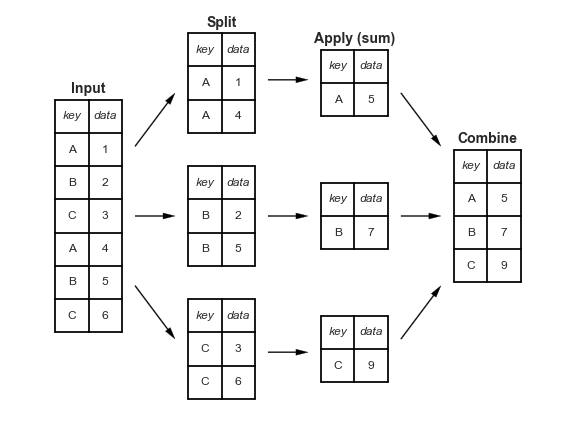
# This makes clear what the ``groupby`` accomplishes:
#
# - The *split* step involves breaking up and grouping a ``DataFrame`` depending on the value of the specified key.
# - The *apply* step involves computing some function, usually an aggregate, transformation, or filtering, within the individual groups.
# - The *combine* step merges the results of these operations into an output array.
#
# While this could certainly be done manually using some combination of the masking, aggregation, and merging commands covered earlier, an important realization is that *the intermediate splits do not need to be explicitly instantiated*. Rather, the ``GroupBy`` can (often) do this in a single pass over the data, updating the sum, mean, count, min, or other aggregate for each group along the way.
# The power of the ``GroupBy`` is that it abstracts away these steps: the user need not think about *how* the computation is done under the hood, but rather thinks about the *operation as a whole*.
#
#
# As a concrete example, let's take a look at using Pandas for the computation shown in this diagram:
# In[156]:
df = pd.DataFrame({'key': ['A', 'B', 'C', 'A', 'B', 'C'],
'data': range(6)}, columns=['key', 'data'])
df
# The most basic split-apply-combine operation can be computed with the ``groupby()`` method of ``DataFrame``s, passing the name of the desired key column:
# In[157]:
df.groupby('key')
# Notice that what is returned is not a set of ``DataFrame``s, but a ``DataFrameGroupBy`` object.
# This object is where the magic is: you can think of it as a special view of the ``DataFrame``, which is poised to dig into the groups but does no actual computation until the aggregation is applied.
# This _lazy evaluation_ approach means that common aggregates can be implemented very efficiently in a way that is almost transparent to the user.
# To produce a result, we can apply an aggregate to this ``DataFrameGroupBy`` object, which will perform the appropriate apply/combine steps to produce the desired result:
# In[158]:
df.groupby('key').sum()
# In[159]:
type(_)
# The ``sum()`` method is just one possibility here; you can apply virtually any common Pandas or NumPy aggregation function, as well as virtually any valid ``DataFrame`` operation.
# ### The GroupBy object
#
# The ``GroupBy`` object is a very flexible abstraction.
# In many ways, you can simply treat it as if it's a collection of ``DataFrame``s, and it does the difficult things under the hood. Let's see some examples using the Planets data.
#
# Perhaps the most important operations made available by a ``GroupBy`` are *aggregate*, *filter*, *transform*, and *apply* but before that let's introduce some of the other functionality that can be used with the basic ``GroupBy`` operation.
# #### Column indexing
#
# The ``GroupBy`` object supports column indexing in the same way as the ``DataFrame``, and returns a modified ``GroupBy`` object:
# In[80]:
planets.groupby('method')
# In[81]:
planets.groupby('method')['orbital_period']
# Here we've selected a particular ``Series`` group from the original ``DataFrame`` group by reference to its column name. As with the ``GroupBy`` object, no computation is done until we call some aggregate on the object:
# In[82]:
planets.groupby('method')['orbital_period'].median()
# #### Iteration over groups
#
# The ``GroupBy`` object supports direct iteration over the groups, returning each group as a ``Series`` or ``DataFrame``:
# In[83]:
for (method, group) in planets.groupby('method'):
print("{0:30s} shape={1}".format(method, group.shape))
# #### Dispatch methods
#
# Through some Python class magic, any method not explicitly implemented by the ``GroupBy`` object will be passed through and called on the groups, whether they are ``DataFrame`` or ``Series`` objects.
# For example, you can use the ``describe()`` method of ``DataFrame``s to perform a set of aggregations that describe each group in the data:
# In[85]:
planets.groupby('method')['year'].describe()
# Looking at this table helps us to better understand the data: for example, the vast majority of planets have been discovered by the Radial Velocity and Transit methods, though the latter only became common (due to new, more accurate telescopes) in the last decade.
# The newest methods seem to be Transit Timing Variation and Orbital Brightness Modulation, which were not used to discover a new planet until 2011.
#
# This is just one example of the utility of dispatch methods.
# Notice that they are applied *to each individual group*, and the results are then combined within ``GroupBy`` and returned.
# Again, any valid ``DataFrame``/``Series`` method can be used on the corresponding ``GroupBy`` object, which allows for some very flexible and powerful operations!
# ### Aggregate, filter, transform, apply
#
# ``GroupBy`` objects have ``aggregate()``, ``filter()``, ``transform()``, and ``apply()`` methods that efficiently implement a variety of useful operations before combining the grouped data.
# In[86]:
rng = np.random.RandomState(0)
df = pd.DataFrame({'key': ['A', 'B', 'C', 'A', 'B', 'C'],
'data1': range(6),
'data2': rng.randint(0, 10, 6)},
columns = ['key', 'data1', 'data2'])
df
# #### Aggregation
#
# We're now familiar with ``GroupBy`` aggregations with ``sum()``, ``median()``, and the like, but the ``aggregate()`` method allows for even more flexibility.
# It can take a string, a function, or a list thereof, and compute all the aggregates at once.
# In[88]:
df.groupby('key').aggregate([min, np.median, max])
# #### Filtering
#
# A filtering operation allows you to drop data based on the group properties.
# For example, we might want to keep all groups in which the standard deviation is larger than some critical value:
# In[91]:
def filter_func(x):
return x['data2'].std() > 4
display('df', "df.groupby('key').std()", "df.groupby('key').filter(filter_func)")
# #### Transformation
#
# While aggregation must return a reduced version of the data, transformation can return some transformed version of the full data to recombine.
# For such a transformation, the output is the same shape as the input.
# In[92]:
df.groupby('key').transform(lambda x: x - x.mean())
# #### The apply() method
#
# The ``apply()`` method lets you apply an arbitrary function to the group results.
# The function should take a ``DataFrame``, and return either a Pandas object (e.g., ``DataFrame``, ``Series``) or a scalar; the combine operation will be tailored to the type of output returned.
# In[93]:
def norm_by_data2(x):
# x is a DataFrame of group values
x['data1'] /= x['data2'].sum()
return x
display('df', "df.groupby('key').apply(norm_by_data2)")
# ### Specifying the split key
#
# In the simple examples presented before, we split the ``DataFrame`` on a single column name.
# This is just one of many options by which the groups can be defined, and we'll go through some other options for group specification here.
# #### A list, array, series, or index providing the grouping keys
#
# The key can be any series or list with a length matching that of the ``DataFrame``:
# In[94]:
L = [0, 1, 0, 1, 2, 0]
display('df', 'df.groupby(L).sum()')
# Of course, this means there's another, more verbose way of accomplishing the ``df.groupby('key')`` from before:
# In[95]:
display('df', "df.groupby(df['key']).sum()")
# #### A dictionary or series mapping index to group
#
# Another method is to provide a dictionary that maps index values to the group keys:
# In[96]:
df2 = df.set_index('key')
mapping = {'A': 'vowel', 'B': 'consonant', 'C': 'consonant'}
display('df2', 'df2.groupby(mapping).sum()')
# #### Any Python function
#
# Similar to mapping, you can pass any Python function that will input the index value and output the group:
# In[97]:
display('df2', 'df2.groupby(str.lower).mean()')
# #### A list of valid keys
#
# Further, any of the preceding key choices can be combined to group on a multi-index:
# In[98]:
df2.groupby([str.lower, mapping]).mean()
# ### Grouping example
#
# As an example of this, in a couple lines of Python code we can put all these together and count discovered planets by method and by decade:
# In[99]:
decade = 10 * (planets['year'] // 10)
decade = decade.astype(str) + 's'
decade.name = 'decade'
planets.groupby(['method', decade])['number'].sum().unstack().fillna(0)
# This shows the power of combining many of the operations we've discussed up to this point when looking at realistic datasets.
# We immediately gain a coarse understanding of when and how planets have been discovered over the past several decades!
# # Pivot Tables
#
# We have seen how the ``GroupBy`` abstraction lets us explore relationships within a dataset.
# A *pivot table* is a similar operation that is commonly seen in spreadsheets and other programs that operate on tabular data:
# - The pivot table takes simple column-wise data as input, and groups the entries into a two-dimensional table that provides a multidimensional summarization of the data.
# - The difference between pivot tables and ``GroupBy`` can sometimes cause confusion; it helps me to think of pivot tables as essentially a *multidimensional* version of ``GroupBy`` aggregation.
# - That is, you split-apply-combine, but both the split and the combine happen across not a one-dimensional index, but across a two-dimensional grid.
# ## Motivating Pivot Tables
#
# We'll use the database of passengers on the *Titanic*, available through the Seaborn library:
# In[101]:
import seaborn as sns
titanic = sns.load_dataset('titanic')
titanic.head()
# ## Pivot Tables by Hand
#
# To start learning more about this data, we might begin by grouping according to gender, survival status, or some combination thereof.
# If you have read the previous section, you might be tempted to apply a ``GroupBy`` operation–for example, let's look at survival rate by gender:
# In[102]:
titanic.groupby('sex')[['survived']].mean()
# This immediately gives us some insight: overall, three of every four females on board survived, while only one in five males survived.
# This is useful, but we might like to go one step deeper and look at survival by both sex and, say, class.
# Using the vocabulary of ``GroupBy``, we might proceed using something like this:
# we *group by* class and gender, *select* survival, *apply* a mean aggregate, *combine* the resulting groups, and then *unstack* the hierarchical index to reveal the hidden multidimensionality. In code:
# In[103]:
titanic.groupby(['sex', 'class'])['survived'].aggregate('mean').unstack()
# This gives us a better idea of how both gender and class affected survival, but the code is starting to look a bit garbled.
# While each step of this pipeline makes sense in light of the tools we've previously discussed, the long string of code is not particularly easy to read or use.
# This two-dimensional ``GroupBy`` is common enough that Pandas includes a convenience routine, ``pivot_table``, which succinctly handles this type of multi-dimensional aggregation.
# ## Pivot Table Syntax
#
# Here is the equivalent to the preceding operation using the ``pivot_table`` method of ``DataFrame``s:
# In[104]:
titanic.pivot_table('survived', index='sex', columns='class')
# This is eminently more readable than the ``groupby`` approach, and produces the same result.
# As you might expect of an early 20th-century transatlantic cruise, the survival gradient favors both women and higher classes.
# First-class women survived with near certainty (hi, Rose!), while only one in ten third-class men survived (sorry, Jack!).
# ### Multi-level pivot tables
#
# Just as in the ``GroupBy``, the grouping in pivot tables can be specified with multiple levels, and via a number of options.
# For example, we might be interested in looking at age as a third dimension.
# We'll bin the age using the ``pd.cut`` function:
# In[105]:
age = pd.cut(titanic['age'], [0, 18, 80])
titanic.pivot_table('survived', ['sex', age], 'class')
# We can apply the same strategy when working with the columns as well; let's add info on the fare paid using ``pd.qcut`` to automatically compute quantiles:
# In[106]:
fare = pd.qcut(titanic['fare'], 2)
titanic.pivot_table('survived', ['sex', age], [fare, 'class'])
# The result is a four-dimensional aggregation with hierarchical indices, shown in a grid demonstrating the relationship between the values.
# ### Additional pivot table options
#
# The full call signature of the ``pivot_table`` method of ``DataFrame``s is as follows:
#
# ```python
# # call signature as of Pandas 0.18
# DataFrame.pivot_table(data, values=None, index=None, columns=None,
# aggfunc='mean', fill_value=None, margins=False,
# dropna=True, margins_name='All')
# ```
#
# We've already seen examples of the first three arguments; here we'll take a quick look at the remaining ones.
# Two of the options, ``fill_value`` and ``dropna``, have to do with missing data and are fairly straightforward; we will not show examples of them here.
#
# The ``aggfunc`` keyword controls what type of aggregation is applied, which is a mean by default.
# As in the GroupBy, the aggregation specification can be a string representing one of several common choices (e.g., ``'sum'``, ``'mean'``, ``'count'``, ``'min'``, ``'max'``, etc.) or a function that implements an aggregation (e.g., ``np.sum()``, ``min()``, ``sum()``, etc.).
# Additionally, it can be specified as a dictionary mapping a column to any of the above desired options:
# In[107]:
titanic.pivot_table(index='sex', columns='class',
aggfunc={'survived':sum, 'fare':'mean'})
# Notice also here that we've omitted the ``values`` keyword; when specifying a mapping for ``aggfunc``, this is determined automatically.
# At times it's useful to compute totals along each grouping.
# This can be done via the ``margins`` keyword:
# In[108]:
titanic.pivot_table('survived', index='sex', columns='class', margins=True)
# Here this automatically gives us information about the class-agnostic survival rate by gender, the gender-agnostic survival rate by class, and the overall survival rate of 38%.
# The margin label can be specified with the ``margins_name`` keyword, which defaults to ``"All"``.
# ## Example: Birthrate Data
#
# As a more interesting example, let's take a look at the freely available data on births in the United States, provided by the Centers for Disease Control (CDC).
# This data can be found at https://raw.githubusercontent.com/jakevdp/data-CDCbirths/master/births.csv:
# In[109]:
get_ipython().system('curl -O https://raw.githubusercontent.com/jakevdp/data-CDCbirths/master/births.csv')
# In[111]:
births = pd.read_csv('data/births.csv')
births.describe()
# Taking a look at the data, we see that it's relatively simple–it contains the number of births grouped by date and gender:
# In[112]:
births.head()
# We can start to understand this data a bit more by using a pivot table.
# Let's add a decade column, and take a look at male and female births as a function of decade:
# In[113]:
births['decade'] = 10 * (births['year'] // 10)
births.pivot_table('births', index='decade', columns='gender', aggfunc='sum')
# We immediately see that male births outnumber female births in every decade.
# To see this trend a bit more clearly, we can use the built-in plotting tools in Pandas to visualize the total number of births by year:
# In[114]:
get_ipython().run_line_magic('matplotlib', 'inline')
import matplotlib.pyplot as plt
sns.set() # use Seaborn styles
births.pivot_table('births', index='year', columns='gender', aggfunc='sum').plot()
plt.ylabel('total births per year');
# With a simple pivot table and ``plot()`` method, we can immediately see the annual trend in births by gender. By eye, it appears that over the past 50 years male births have outnumbered female births by around 5%.
# ### Further data exploration
#
# Though this doesn't necessarily relate to the pivot table, there are a few more interesting features we can pull out of this dataset using the Pandas tools covered up to this point.
# We must start by cleaning the data a bit, removing outliers caused by mistyped dates (e.g., June 31st) or missing values (e.g., June 99th).
# One easy way to remove these all at once is to cut outliers; we'll do this via a robust sigma-clipping operation:
# In[115]:
quartiles = np.percentile(births['births'], [25, 50, 75])
mu = quartiles[1]
sig = 0.74 * (quartiles[2] - quartiles[0])
# This final line is a robust estimate of the sample mean, where the 0.74 comes from the interquartile range of a Gaussian distribution.
# With this we can use the ``query()`` method to filter-out rows with births outside these values:
# In[116]:
births = births.query('(births > @mu - 5 * @sig) & (births < @mu + 5 * @sig)')
# Next we set the ``day`` column to integers; previously it had been a string because some columns in the dataset contained the value ``'null'``:
# In[117]:
# set 'day' column to integer; it originally was a string due to nulls
births['day'] = births['day'].astype(int)
# Finally, we can combine the day, month, and year to create a Date index.
# This allows us to quickly compute the weekday corresponding to each row:
# In[118]:
# create a datetime index from the year, month, day
births.index = pd.to_datetime(10000 * births.year +
100 * births.month +
births.day, format='%Y%m%d')
births['dayofweek'] = births.index.dayofweek
# In[120]:
import matplotlib.pyplot as plt
import matplotlib as mpl
births.pivot_table('births', index='dayofweek',
columns='decade', aggfunc='mean').plot()
plt.gca().set_xticklabels(['Mon', 'Tues', 'Wed', 'Thurs', 'Fri', 'Sat', 'Sun'])
plt.ylabel('mean births by day');
# Apparently births are slightly less common on weekends than on weekdays! Note that the 1990s and 2000s are missing because the CDC data contains only the month of birth starting in 1989.
# Another intersting view is to plot the mean number of births by the day of the *year*.
# Let's first group the data by month and day separately:
# In[133]:
births_by_date = births.pivot_table('births', [births.index.month, births.index.day])
births_by_date.head()
# The result is a multi-index over months and days.
# To make this easily plottable, let's turn these months and days into a date by associating them with a dummy year variable (making sure to choose a leap year so February 29th is correctly handled!)
# In[134]:
from datetime import datetime
births_by_date.index = [datetime(2012, month, day)
for (month, day) in births_by_date.index]
births_by_date.head()
# Focusing on the month and day only, we now have a time series reflecting the average number of births by date of the year.
# From this, we can use the ``plot`` method to plot the data. It reveals some interesting trends:
# In[135]:
fig, ax = plt.subplots(figsize=(12, 4))
births_by_date.plot(ax=ax);
# In particular, the striking feature of this graph is the dip in birthrate on US holidays (e.g., Independence Day, Labor Day, Thanksgiving, Christmas, New Year's Day) although this likely reflects trends in scheduled/induced births rather than some deep psychosomatic effect on natural births.
#
# Looking at this short example, you can see that many of the Python and Pandas tools we've seen to this point can be combined and used to gain insight from a variety of datasets.
# # Working with Time Series
#
# Pandas was developed in the context of financial modeling, so as you might expect, it contains a fairly extensive set of tools for working with dates, times, and time-indexed data.
# Date and time data comes in a few flavors:
#
# - *Time stamps* reference particular moments in time (e.g., July 4th, 2015 at 7:00am).
# - *Time intervals* and *periods* reference a length of time between a particular beginning and end point; for example, the year 2015. Periods usually reference a special case of time intervals in which each interval is of uniform length and does not overlap (e.g., 24 hour-long periods comprising days).
# - *Time deltas* or *durations* reference an exact length of time (e.g., a duration of 22.56 seconds).
# ## Dates and Times in Python
#
# The Python world has a number of available representations of dates, times, deltas, and timespans.
# While the time series tools provided by Pandas tend to be the most useful for data science applications, it is helpful to see their relationship to other packages used in Python.
# ### Native Python dates and times: ``datetime`` and ``dateutil``
#
# Python's basic objects for working with dates and times reside in the built-in ``datetime`` module.
# Along with the third-party ``dateutil`` module, you can use it to quickly perform a host of useful functionalities on dates and times:
# In[237]:
from datetime import datetime
datetime(year=2015, month=7, day=4)
# Or, using the ``dateutil`` module, you can parse dates from a variety of string formats:
# In[238]:
from dateutil import parser
date = parser.parse("4th of July, 2015")
date
# Once you have a ``datetime`` object, you can do things like printing the day of the week:
# In[239]:
date.strftime('%A')
# A related package to be aware of is [``pytz``](http://pytz.sourceforge.net/), which contains tools for working with the most migrane-inducing piece of time series data: time zones.
#
# The power of ``datetime`` and ``dateutil`` lie in their flexibility and easy syntax: you can use these objects and their built-in methods to easily perform nearly any operation you might be interested in.
# Where they break down is when you wish to work with large arrays of dates and times:
# just as lists of Python numerical variables are suboptimal compared to NumPy-style typed numerical arrays, lists of Python datetime objects are suboptimal compared to typed arrays of encoded dates.
# ### Typed arrays of times: NumPy's ``datetime64``
#
# The weaknesses of Python's datetime format inspired the NumPy team to add a set of native time series data type to NumPy.
# The ``datetime64`` dtype encodes dates as 64-bit integers, and thus allows arrays of dates to be represented very compactly.
# In[240]:
date = np.array('2015-07-04', dtype=np.datetime64)
date
# Once we have this date formatted, however, we can quickly do vectorized operations on it:
# In[241]:
date + np.arange(12)
# Because of the uniform type in NumPy ``datetime64`` arrays, this type of operation can be accomplished much more quickly than if we were working directly with Python's ``datetime`` objects, especially as arrays get large.
#
# One detail of the ``datetime64`` and ``timedelta64`` objects is that they are built on a *fundamental time unit*.
# Because the ``datetime64`` object is limited to 64-bit precision, the range of encodable times is $2^{64}$ times this fundamental unit. In other words, ``datetime64`` imposes a trade-off between *time resolution* and *maximum time span*.
# If you want a time resolution of one nanosecond, you only have enough information to encode a range of $2^{64}$ nanoseconds, or just under 600 years:
# In[242]:
np.datetime64('2015-07-04') # a day-based datetime
# In[243]:
np.datetime64('2015-07-04 12:00') # a minute-based datetime
# In[244]:
np.datetime64('2015-07-04 12:59:59.50', 'ns') # a nanosecond-based datetiem
# The following table lists the available format codes along with the relative and absolute timespans that they can encode:
#
# |Code | Meaning | Time span (relative) | Time span (absolute) |
# |--------|-------------|----------------------|------------------------|
# | ``Y`` | Year | ± 9.2e18 years | [9.2e18 BC, 9.2e18 AD] |
# | ``M`` | Month | ± 7.6e17 years | [7.6e17 BC, 7.6e17 AD] |
# | ``W`` | Week | ± 1.7e17 years | [1.7e17 BC, 1.7e17 AD] |
# | ``D`` | Day | ± 2.5e16 years | [2.5e16 BC, 2.5e16 AD] |
# | ``h`` | Hour | ± 1.0e15 years | [1.0e15 BC, 1.0e15 AD] |
# | ``m`` | Minute | ± 1.7e13 years | [1.7e13 BC, 1.7e13 AD] |
# | ``s`` | Second | ± 2.9e12 years | [ 2.9e9 BC, 2.9e9 AD] |
# | ``ms`` | Millisecond | ± 2.9e9 years | [ 2.9e6 BC, 2.9e6 AD] |
# | ``us`` | Microsecond | ± 2.9e6 years | [290301 BC, 294241 AD] |
# | ``ns`` | Nanosecond | ± 292 years | [ 1678 AD, 2262 AD] |
# | ``ps`` | Picosecond | ± 106 days | [ 1969 AD, 1970 AD] |
# | ``fs`` | Femtosecond | ± 2.6 hours | [ 1969 AD, 1970 AD] |
# | ``as`` | Attosecond | ± 9.2 seconds | [ 1969 AD, 1970 AD] |
# ### Dates and times in pandas: best of both worlds
#
# Pandas builds upon all the tools just discussed to provide a ``Timestamp`` object, which combines the ease-of-use of ``datetime`` and ``dateutil`` with the efficient storage and vectorized interface of ``numpy.datetime64``.
# From a group of these ``Timestamp`` objects, Pandas can construct a ``DatetimeIndex`` that can be used to index data in a ``Series`` or ``DataFrame``:
# In[245]:
date = pd.to_datetime("4th of July, 2015")
date
# In[246]:
date.strftime('%A')
# In[247]:
date + pd.to_timedelta(np.arange(12), 'D') # do NumPy-style vectorized operations directly on this same object
# ## Pandas Time Series: Indexing by Time
#
# Where the Pandas time series tools really become useful is when you begin to *index data by timestamps*:
# In[249]:
index = pd.DatetimeIndex(['2014-07-04', '2014-08-04', '2015-07-04', '2015-08-04'])
data = pd.Series([0, 1, 2, 3], index=index)
data
# Now that we have this data in a ``Series``, we can make use of any of the ``Series`` indexing patterns passing values that can be coerced into dates:
# In[250]:
data['2014-07-04':'2015-07-04']
# In[251]:
data['2015'] # additional special date-only indexing operations
# ## Pandas Time Series Data Structures
#
# The fundamental Pandas data structures for working with time series data:
#
# - For *time stamps*, Pandas provides the ``Timestamp`` type. As mentioned before, it is essentially a replacement for Python's native ``datetime``, but is based on the more efficient ``numpy.datetime64`` data type. The associated Index structure is ``DatetimeIndex``.
# - For *time Periods*, Pandas provides the ``Period`` type. This encodes a fixed-frequency interval based on ``numpy.datetime64``. The associated index structure is ``PeriodIndex``.
# - For *time deltas* or *durations*, Pandas provides the ``Timedelta`` type. ``Timedelta`` is a more efficient replacement for Python's native ``datetime.timedelta`` type, and is based on ``numpy.timedelta64``. The associated index structure is ``TimedeltaIndex``.
# The most fundamental of these date/time objects are the ``Timestamp`` and ``DatetimeIndex`` objects.
# While these class objects can be invoked directly, it is more common to use the ``pd.to_datetime()`` function, which can parse a wide variety of formats.
# Passing a single date to ``pd.to_datetime()`` yields a ``Timestamp``; passing a series of dates by default yields a ``DatetimeIndex``:
# In[252]:
dates = pd.to_datetime([datetime(2015, 7, 3), '4th of July, 2015',
'2015-Jul-6', '07-07-2015', '20150708'])
dates
# Any ``DatetimeIndex`` can be converted to a ``PeriodIndex`` with the ``to_period()`` function with the addition of a frequency code; here we'll use ``'D'`` to indicate daily frequency:
# In[254]:
dates.to_period('D')
# In[255]:
dates - dates[0] # A ``TimedeltaIndex`` is createdwhen subtracting
# ### Regular sequences: ``pd.date_range()``
#
# To make the creation of regular date sequences more convenient, Pandas offers a few functions for this purpose: ``pd.date_range()`` for timestamps, ``pd.period_range()`` for periods, and ``pd.timedelta_range()`` for time deltas:
# In[256]:
pd.date_range('2015-07-03', '2015-07-10') # by default, the frequency is one day
# In[257]:
pd.date_range('2015-07-03', periods=8)
# In[258]:
pd.date_range('2015-07-03', periods=8, freq='H')
# In[260]:
pd.period_range('2015-07', periods=8, freq='M')
# In[261]:
pd.timedelta_range(0, periods=10, freq='H')
# ## Frequencies and Offsets
#
# Fundamental to these Pandas time series tools is the concept of a frequency or date offset.
# Just as we saw the ``D`` (day) and ``H`` (hour) codes above, we can use such codes to specify any desired frequency spacing:
#
# | Code | Description | Code | Description |
# |--------|---------------------|--------|----------------------|
# | ``D`` | Calendar day | ``B`` | Business day |
# | ``W`` | Weekly | | |
# | ``M`` | Month end | ``BM`` | Business month end |
# | ``Q`` | Quarter end | ``BQ`` | Business quarter end |
# | ``A`` | Year end | ``BA`` | Business year end |
# | ``H`` | Hours | ``BH`` | Business hours |
# | ``T`` | Minutes | | |
# | ``S`` | Seconds | | |
# | ``L`` | Milliseonds | | |
# | ``U`` | Microseconds | | |
# | ``N`` | nanoseconds | | |
# The monthly, quarterly, and annual frequencies are all marked at the end of the specified period.
# By adding an ``S`` suffix to any of these, they instead will be marked at the beginning:
#
# | Code | Description || Code | Description |
# |---------|------------------------||---------|------------------------|
# | ``MS`` | Month start ||``BMS`` | Business month start |
# | ``QS`` | Quarter start ||``BQS`` | Business quarter start |
# | ``AS`` | Year start ||``BAS`` | Business year start |
# Additionally, you can change the month used to mark any quarterly or annual code by adding a three-letter month code as a suffix:
#
# - ``Q-JAN``, ``BQ-FEB``, ``QS-MAR``, ``BQS-APR``, etc.
# - ``A-JAN``, ``BA-FEB``, ``AS-MAR``, ``BAS-APR``, etc.
#
# In the same way, the split-point of the weekly frequency can be modified by adding a three-letter weekday code:
#
# - ``W-SUN``, ``W-MON``, ``W-TUE``, ``W-WED``, etc.
#
# On top of this, codes can be combined with numbers to specify other frequencies.
# For example, for a frequency of 2 hours 30 minutes, we can combine the hour (``H``) and minute (``T``) codes as follows:
# In[262]:
pd.timedelta_range(0, periods=9, freq="2H30T")
# All of these short codes refer to specific instances of Pandas time series offsets, which can be found in the ``pd.tseries.offsets`` module.
# For example, we can create a business day offset directly as follows:
# In[263]:
from pandas.tseries.offsets import BDay
pd.date_range('2015-07-01', periods=5, freq=BDay())
# ## Resampling, Shifting, and Windowing
#
# The ability to use dates and times as indices to intuitively organize and access data is an important piece of the Pandas time series tools. The benefits of indexed data in general (automatic alignment during operations, intuitive data slicing and access, etc.) still apply, and Pandas provides several additional time series-specific operations.
#
# We will take a look at a few of those here, using some stock price data as an example.
# Because Pandas was developed largely in a finance context, it includes some very specific tools for financial data.
#
# For example, the accompanying ``pandas-datareader`` package (installable via ``pip install pandas-datareader``), knows how to import financial data from a number of available sources, including Yahoo finance, Google Finance, and others.
# Download some data (**ADD A DESCRIPTION FOR IT**)
# In[21]:
from pandas_datareader import data
goog = data.DataReader('VIXCLS', start='2004', end='2016', data_source='fred')
goog.head()
# In[22]:
goog = goog['VIXCLS'] # for simplicity consider its sole column
# In[23]:
get_ipython().run_line_magic('matplotlib', 'inline')
import matplotlib.pyplot as plt
import seaborn; seaborn.set()
goog.plot();
# ### Resampling and converting frequencies
#
# One common need for time series data is resampling at a higher or lower frequency.
# This can be done using the ``resample()`` method, or the much simpler ``asfreq()`` method.
# The primary difference between the two is that ``resample()`` is fundamentally a *data aggregation*, while ``asfreq()`` is fundamentally a *data selection*.
# Let's compare what the two return when we down-sample the data; we will resample the data at the end of business year:
# In[24]:
goog.plot(alpha=0.5, style='-')
goog.resample('BA').mean().plot(style=':')
goog.asfreq('BA').plot(style='--');
plt.legend(['input', 'resample', 'asfreq'], loc='upper left');
# Notice the difference: at each point, ``resample`` reports the *average of the previous year*, while ``asfreq`` reports the *value at the end of the year*.
# For up-sampling, ``resample()`` and ``asfreq()`` are largely equivalent, though resample has many more options available.
# In this case, the default for both methods is to leave the up-sampled points empty, that is, filled with NA values.
# Just as with the ``pd.fillna()`` function discussed previously, ``asfreq()`` accepts a ``method`` argument to specify how values are imputed.
# We resample the business day data at a daily frequency (i.e., including weekends):
# In[25]:
fig, ax = plt.subplots(2, sharex=True)
data = goog.iloc[:10]
data.asfreq('D').plot(ax=ax[0], marker='o')
data.asfreq('D', method='bfill').plot(ax=ax[1], style='-o')
data.asfreq('D', method='ffill').plot(ax=ax[1], style='--o')
ax[1].legend(["back-fill", "forward-fill"]);
# The top panel is the default: non-business days are left as NA values and do not appear on the plot.
# The bottom panel shows the differences between two strategies for filling the gaps: forward-filling and backward-filling.
# ### Time-shifts
#
# Another common time series-specific operation is shifting of data in time.
# Pandas has two closely related methods for computing this: ``shift()`` and ``tshift()``
# In short, the difference between them is that ``shift()`` *shifts the data*, while ``tshift()`` *shifts the index*.
# In both cases, the shift is specified in multiples of the frequency.
#
# Here we will both ``shift()`` and ``tshift()`` by 900 days;
# In[28]:
fig, ax = plt.subplots(3, sharey=True)
# apply a frequency to the data
goog = goog.asfreq('D', method='pad')
goog.plot(ax=ax[0])
goog.shift(900).plot(ax=ax[1])
goog.tshift(900).plot(ax=ax[2])
# legends and annotations
local_max = pd.to_datetime('2007-11-05')
offset = pd.Timedelta(900, 'D')
ax[0].legend(['input'], loc=2)
ax[0].get_xticklabels()[2].set(weight='heavy', color='red')
ax[0].axvline(local_max, alpha=0.3, color='red')
ax[1].legend(['shift(900)'], loc=2)
ax[1].get_xticklabels()[2].set(weight='heavy', color='red')
ax[1].axvline(local_max + offset, alpha=0.3, color='red')
ax[2].legend(['tshift(900)'], loc=2)
ax[2].get_xticklabels()[1].set(weight='heavy', color='red')
ax[2].axvline(local_max + offset, alpha=0.3, color='red');
# We see here that ``shift(900)`` shifts the *data* by 900 days, pushing some of it off the end of the graph (and leaving NA values at the other end), while ``tshift(900)`` shifts the *index values* by 900 days.
#
# A common context for this type of shift is in computing differences over time. For example, we use shifted values to compute the one-year return on investment for Google stock over the course of the dataset:
# In[29]:
ROI = 100 * (goog.tshift(-365) / goog - 1)
ROI.plot()
plt.ylabel('% Return on Investment');
# This helps us to see the overall trend in Google stock: thus far, the most profitable times to invest in Google have been (unsurprisingly, in retrospect) shortly after its IPO, and in the middle of the 2009 recession.
# ### Rolling windows
#
# Rolling statistics are a third type of time series-specific operation implemented by Pandas.
# These can be accomplished via the ``rolling()`` attribute of ``Series`` and ``DataFrame`` objects, which returns a view similar to what we saw with the ``groupby`` operation (see [Aggregation and Grouping](03.08-Aggregation-and-Grouping.ipynb)).
# This rolling view makes available a number of aggregation operations by default.
# For example, here is the one-year centered rolling mean and standard deviation of the Google stock prices:
# In[34]:
rolling = goog.rolling(40, center=True)
data = pd.DataFrame({'input': goog,
'one-year rolling_mean': rolling.mean(),
'one-year rolling_std': rolling.std()})
ax = data.plot(style=['-', '--', ':'])
ax.lines[0].set_alpha(0.3)
# As with group-by operations, the ``aggregate()`` and ``apply()`` methods can be used for custom rolling computations.
# ## Example: Visualizing Seattle Bicycle Counts
#
# As a more involved example of working with some time series data, let's take a look at bicycle counts on Seattle's [Fremont Bridge](http://www.openstreetmap.org/#map=17/47.64813/-122.34965).
# This data comes from an automated bicycle counter, installed in late 2012, which has inductive sensors on the east and west sidewalks of the bridge.
# The hourly bicycle counts can be downloaded from http://data.seattle.gov/; here is the [direct link to the dataset](https://data.seattle.gov/Transportation/Fremont-Bridge-Hourly-Bicycle-Counts-by-Month-Octo/65db-xm6k).
#
# As of summer 2016, the CSV can be downloaded as follows:
# In[37]:
get_ipython().system('curl -o FremontBridge.csv https://data.seattle.gov/api/views/65db-xm6k/rows.csv?accessType=DOWNLOAD')
# Once this dataset is downloaded, we can use Pandas to read the CSV output into a ``DataFrame``.
# We will specify that we want the Date as an index, and we want these dates to be automatically parsed:
# In[41]:
data = pd.read_csv('data/FremontBridge.csv', index_col='Date', parse_dates=True)
data.head()
# We'll further process this dataset by shortening the column names and adding a "Total" column:
# In[50]:
data['Total'] = data["Fremont Bridge Total"]
data.dropna().describe() # have a look at summary statistics
# ### Visualizing the data
#
# We can gain some insight into the dataset by visualizing it:
# In[51]:
get_ipython().run_line_magic('matplotlib', 'inline')
import seaborn; seaborn.set()
# In[52]:
data.plot()
plt.ylabel('Hourly Bicycle Count');
# The ~25,000 hourly samples are far too dense for us to make much sense of.
# We can gain more insight by resampling the data to a coarser grid:
# In[53]:
weekly = data.resample('W').sum()
weekly.plot(style=[':', '--', '-'])
plt.ylabel('Weekly bicycle count');
# This shows us some interesting seasonal trends: as you might expect, people bicycle more in the summer than in the winter, and even within a particular season the bicycle use varies from week to week (likely dependent on weather.
#
# Another way that comes in handy for aggregating the data is to use a rolling mean, utilizing the ``pd.rolling_mean()`` function.
# Here we'll do a 30 day rolling mean of our data, making sure to center the window:
# In[54]:
daily = data.resample('D').sum()
daily.rolling(30, center=True).sum().plot(style=[':', '--', '-'])
plt.ylabel('mean hourly count');
# The jaggedness of the result is due to the hard cutoff of the window.
# We can get a smoother version of a rolling mean using a window function–for example, a Gaussian window.
# The following code specifies both the width of the window (we chose 50 days) and the width of the Gaussian within the window (we chose 10 days):
# In[55]:
daily.rolling(50, center=True,
win_type='gaussian').sum(std=10).plot(style=[':', '--', '-']);
# ### Digging into the data
#
# While these smoothed data views are useful to get an idea of the general trend in the data, they hide much of the interesting structure.
# For example, we might want to look at the average traffic as a function of the time of day; we do this by grouping:
# In[56]:
by_time = data.groupby(data.index.time).mean()
hourly_ticks = 4 * 60 * 60 * np.arange(6)
by_time.plot(xticks=hourly_ticks, style=[':', '--', '-']);
# The hourly traffic is a strongly bimodal distribution, with peaks around 8:00 in the morning and 5:00 in the evening.
# This is likely evidence of a strong component of commuter traffic crossing the bridge.
# This is further evidenced by the differences between the western sidewalk (generally used going toward downtown Seattle), which peaks more strongly in the morning, and the eastern sidewalk (generally used going away from downtown Seattle), which peaks more strongly in the evening.
#
# We also might be curious about how things change based on the day of the week. Again, we can do this with a simple groupby:
# In[57]:
by_weekday = data.groupby(data.index.dayofweek).mean()
by_weekday.index = ['Mon', 'Tues', 'Wed', 'Thurs', 'Fri', 'Sat', 'Sun']
by_weekday.plot(style=[':', '--', '-']);
# This shows a strong distinction between weekday and weekend totals, with around twice as many average riders crossing the bridge on Monday through Friday than on Saturday and Sunday.
# With this in mind, let's do a compound GroupBy and look at the hourly trend on weekdays versus weekends.
# We'll start by grouping by both a flag marking the weekend, and the time of day:
# In[58]:
weekend = np.where(data.index.weekday < 5, 'Weekday', 'Weekend')
by_time = data.groupby([weekend, data.index.time]).mean()
# In[65]:
import matplotlib.pyplot as plt
fig, ax = plt.subplots(1, 2, figsize=(14, 5))
by_time.loc['Weekday'].plot(ax=ax[0], title='Weekdays',
xticks=hourly_ticks, style=[':', '--', '-'])
by_time.loc['Weekend'].plot(ax=ax[1], title='Weekends',
xticks=hourly_ticks, style=[':', '--', '-']);
# The result is very interesting: we see a bimodal commute pattern during the work week, and a unimodal recreational pattern during the weekends.