#!/usr/bin/env python
# coding: utf-8
# + title: Natural Language Processing of German texts - Part 1: Using machine-learning to predict ratings
# + date: 2020-04-10
# + tags: python, NLP, sklearn, classification, machine-learning, tf-idf
# + Slug: german-nlp-binary-text-classification-of-reviews-part1
# + Category: Python
# + Authors: MC
# + Summary: Using a unique German data set containing ratings and comments on doctors, we build a Binary Text Classifier. To do so, we implement a complete machine learning work flow that predicts ratings from comments. In this first part, we start with basic methods. We go through text pre processing, feature creation (TF-IDF), classification and model optimization. Finally, we evaluate our model's ability to predict the sentiment of comments.
# ### Motivation
#
# The domain of Natural Language Processing (NLP) has seen a rapid advancement during the last few years. In particular, 2019 has been a remarkable year. New state of the art results on all relevant benchmarks have been established on a regular basis. In this multi part post we apply and compare several methods of Binary Text Classification, starting with traditional, basic methods and leading to state of the art models. For this, we use a novel German data set that contains hundreds of thousands of comments. They were submitted by patients on an online platform for reviewing doctors. The data also contains ratings so that it can be used to train supervised models in order to predict the rating / sentiment of the comment.
# Most data sets for NLP are in English and the majority of learning resources also focus on English. Hence, the unique data at our hands is valuable for applying NLP methods to German text. Because of its many observations and the fact that it contains labels, it is ideal for applying machine-learning methods.
# Let's take a look at a basic NLP workflow:
#
#
#
# 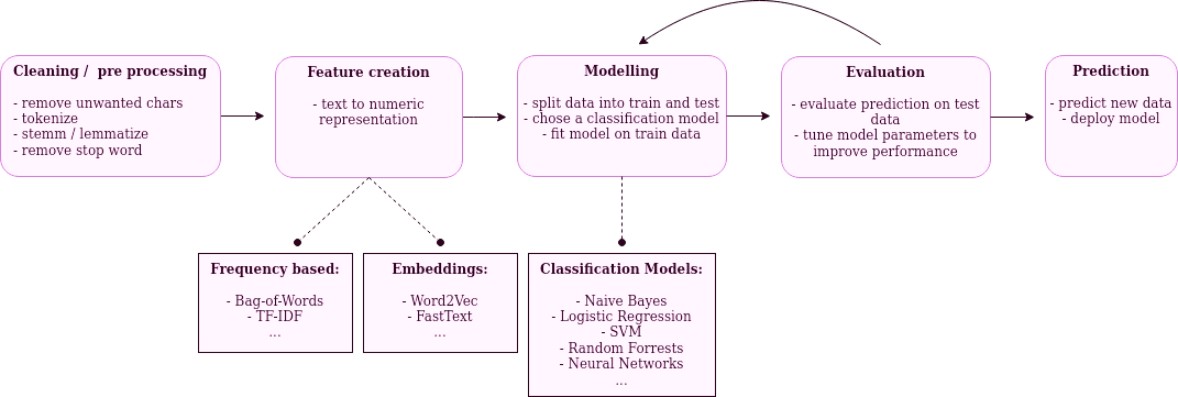 #
# A typical NLP machine-learning workflow (own illustration)
#
#
# A typical NLP machine-learning workflow (own illustration)
#
#
# In the following notebook, we will go through this process step by step. In this first part, we apply frequency based methods for feature creation and compare several classification models. Moreover, we optimize the parameters of our process using a grid search. We'll see that these "traditional" methods already achieve adequate results on our data, that we'll use as a baseline. In follow up posts, we will apply more advanced methods and try to improve on our results in the search for the best performing model. During this journey, we will compare the different methods and discuss their pros and cons.
#
# You can download this notebook or follow along in an interactive version of it on  and
#
and
#  .
# ### The data set
#
# You can take a look at the data on [data.world](https://data.world/mc51/german-language-reviews-of-doctors-by-patients) or directly download it from [here](https://query.data.world/s/v5xl53bs2rgq476vqy7cg7xx2db55y):
# In[ ]:
# store current path and download data there
CURR_PATH = get_ipython().getoutput('pwd')
get_ipython().system('wget -O reviews.zip https://query.data.world/s/v5xl53bs2rgq476vqy7cg7xx2db55y')
get_ipython().system('unzip reviews.zip')
# After unzipping you'll get a csv file.
# Before we open it, let's setup our notebook by loading all relevant modules and setting some options:
# In[91]:
import re
import pickle
import sklearn
import pandas as pd
import numpy as np
import holoviews as hv
import hvplot
import nltk
from bokeh.io import output_notebook
output_notebook()
from hvplot import pandas
from pathlib import Path
#hv.extension("bokeh")
pd.options.display.max_columns = 100
pd.options.display.max_rows = 300
pd.options.display.max_colwidth = 100
np.set_printoptions(threshold=2000)
# In[5]:
from sklearn.model_selection import train_test_split
from sklearn.feature_extraction.text import TfidfVectorizer
from sklearn.linear_model import LogisticRegression
from sklearn.svm import LinearSVC
from sklearn.ensemble import RandomForestClassifier
from sklearn.neural_network import MLPClassifier
from sklearn.pipeline import Pipeline
from sklearn.model_selection import GridSearchCV
from xgboost import XGBClassifier
from nltk.stem.snowball import SnowballStemmer
from nltk.tokenize import word_tokenize
from nltk.corpus import stopwords
# For dealing with text related tasks, we will be using [nltk](https://www.nltk.org). The terrific [scikit-learn](https://scikit-learn.org/) library will be used to handle tasks related to machine learning.
# Now, we can take a peek into the data:
# In[13]:
# Read raw data
FILE_REVIEWS = Path(CURR_PATH[0]) / "german_doctor_reviews.csv"
data = pd.read_csv(FILE_REVIEWS, sep=",", na_values=[""])
data.head(3)
# We'll focus on the comments and the ratings, which range from one to six. The comments are mostly written in proper German using punctuation and don't include emojis. However, as with any real life text data there will be slang, grammatical mistakes, misspellings etc. Also, in some places we find html tags like `
.
# ### The data set
#
# You can take a look at the data on [data.world](https://data.world/mc51/german-language-reviews-of-doctors-by-patients) or directly download it from [here](https://query.data.world/s/v5xl53bs2rgq476vqy7cg7xx2db55y):
# In[ ]:
# store current path and download data there
CURR_PATH = get_ipython().getoutput('pwd')
get_ipython().system('wget -O reviews.zip https://query.data.world/s/v5xl53bs2rgq476vqy7cg7xx2db55y')
get_ipython().system('unzip reviews.zip')
# After unzipping you'll get a csv file.
# Before we open it, let's setup our notebook by loading all relevant modules and setting some options:
# In[91]:
import re
import pickle
import sklearn
import pandas as pd
import numpy as np
import holoviews as hv
import hvplot
import nltk
from bokeh.io import output_notebook
output_notebook()
from hvplot import pandas
from pathlib import Path
#hv.extension("bokeh")
pd.options.display.max_columns = 100
pd.options.display.max_rows = 300
pd.options.display.max_colwidth = 100
np.set_printoptions(threshold=2000)
# In[5]:
from sklearn.model_selection import train_test_split
from sklearn.feature_extraction.text import TfidfVectorizer
from sklearn.linear_model import LogisticRegression
from sklearn.svm import LinearSVC
from sklearn.ensemble import RandomForestClassifier
from sklearn.neural_network import MLPClassifier
from sklearn.pipeline import Pipeline
from sklearn.model_selection import GridSearchCV
from xgboost import XGBClassifier
from nltk.stem.snowball import SnowballStemmer
from nltk.tokenize import word_tokenize
from nltk.corpus import stopwords
# For dealing with text related tasks, we will be using [nltk](https://www.nltk.org). The terrific [scikit-learn](https://scikit-learn.org/) library will be used to handle tasks related to machine learning.
# Now, we can take a peek into the data:
# In[13]:
# Read raw data
FILE_REVIEWS = Path(CURR_PATH[0]) / "german_doctor_reviews.csv"
data = pd.read_csv(FILE_REVIEWS, sep=",", na_values=[""])
data.head(3)
# We'll focus on the comments and the ratings, which range from one to six. The comments are mostly written in proper German using punctuation and don't include emojis. However, as with any real life text data there will be slang, grammatical mistakes, misspellings etc. Also, in some places we find html tags like `
`. Nonetheless, compared to data from Facebook or Twitter this is mostly harmless and probably won't pose too many issues for us. We will deal with all of that in the next step.
# ### Cleaning and pre processing
#
# Having consistent and clean data is fundamental for good modeling results. No matter how sophisticated your model the basic principle is: trash in trash out. When dealing with NLP the cleaning and pre processing can differ depending on which model you intend to use. We will use frequency based representation methods for our text. Thus, we usually want to have a pretty thorough manipulation of the input data:
# In[16]:
nltk.download('punkt')
nltk.download('stopwords')
stemmer = SnowballStemmer("german")
stop_words = set(stopwords.words("german"))
def clean_text(text, for_embedding=False):
"""
- remove any html tags (< /br> often found)
- Keep only ASCII + European Chars and whitespace, no digits
- remove single letter chars
- convert all whitespaces (tabs etc.) to single wspace
if not for embedding (but e.g. tdf-idf):
- all lowercase
- remove stopwords, punctuation and stemm
"""
RE_WSPACE = re.compile(r"\s+", re.IGNORECASE)
RE_TAGS = re.compile(r"<[^>]+>")
RE_ASCII = re.compile(r"[^A-Za-zÀ-ž ]", re.IGNORECASE)
RE_SINGLECHAR = re.compile(r"\b[A-Za-zÀ-ž]\b", re.IGNORECASE)
if for_embedding:
# Keep punctuation
RE_ASCII = re.compile(r"[^A-Za-zÀ-ž,.!? ]", re.IGNORECASE)
RE_SINGLECHAR = re.compile(r"\b[A-Za-zÀ-ž,.!?]\b", re.IGNORECASE)
text = re.sub(RE_TAGS, " ", text)
text = re.sub(RE_ASCII, " ", text)
text = re.sub(RE_SINGLECHAR, " ", text)
text = re.sub(RE_WSPACE, " ", text)
word_tokens = word_tokenize(text)
words_tokens_lower = [word.lower() for word in word_tokens]
if for_embedding:
# no stemming, lowering and punctuation / stop words removal
words_filtered = word_tokens
else:
words_filtered = [
stemmer.stem(word) for word in words_tokens_lower if word not in stop_words
]
text_clean = " ".join(words_filtered)
return text_clean
# The `clean_text` function takes a string input and applies a bunch of manipulations to it (described in the code). Check out this example:
# In[17]:
clean_text("Python ist die beste Programmiersprache der Welt.")
# This transformation has a few benefits. Removing characters and words that don't hold much meaning reduces the size of our data. Moreover, it can improve prediction performance when modeling by lowering the noise in the data. This is because e.g. stop words like prepositions or punctuation won't allow our model to extract additional information / meaning (at least when using simple models). By stemming and lower casing words we make sure that similar words are treated identically. Thus, we can improve model performance again by increasing the number of relevant data points.
# Let's apply this to our data:
# In[18]:
get_ipython().run_cell_magic('time', '', '# Clean Comments\ndata["comment_clean"] = data.loc[data["comment"].str.len() > 20, "comment"]\ndata["comment_clean"] = data["comment_clean"].map(\n lambda x: clean_text(x, for_embedding=False) if isinstance(x, str) else x\n)\n')
# For our classification task, we want to be able to recognize whether a comment has a positive or negative sentiment. We make use of the ratings that come alongside with all comments. Naturally, we assume that good ratings (1-2) convey a positive message while low ratings (5-6) convey a negative one. We exclude neutral ratings, so that our task becomes a binary classification. Keeping them would turn the task into a multi label classification problem, requiring a slightly different modeling approach.
# In[19]:
# Create binary grade, class 1-2 or 5-6 = good or bad
data["grade_bad"] = 0
data.loc[data["rating"] >= 3, "grade_bad"] = np.NaN
data.loc[data["rating"] >= 5, "grade_bad"] = 1
# Drop when any of x missing
data = data[(data["comment_clean"] != "") & (data["comment_clean"] != "null")]
data = data.dropna(
axis="index", subset=["grade_bad", "comment", "comment_clean"]
).reset_index(drop=True)
# In[20]:
# data.to_csv("../../data/processed/comments_clean.csv", index=False)
data_clean = data.copy()
# data_clean = pd.read_csv("../../data/processed/comments_clean.csv")
# These steps conclude the cleaning and pre processing. In result, we get this:
# In[21]:
data_clean.head(3)
# The cleaned comments are much more concise because their original sentence structure and their words have been altered severely. Although the meaning can still be grasped, humans will probably have a harder time understanding these sentences. In contrast, many classification approaches greatly benefit from this simplification. Some reasons for that have been mentioned above. Basically, it boils down to the fact that we try to keep only informative pieces of text that aid the **specific model** we intend to apply to the task. In this case, we will use simple models that benefit from less complexity. However, more advanced models are able to extract information from more complex features. Thus, they can perform better with less simplification of the input texts. We'll take a look at that in an upcoming post.
# ### Descriptive analysis
#
# Even though we deal with texts, we should still use some descriptive analysis to get a better understanding of the data:
# In[22]:
from bokeh.models import NumeralTickFormatter
# Word Frequency of most common words
word_freq = pd.Series(" ".join(data_clean["comment_clean"]).split()).value_counts()
word_freq[1:40].rename("Word frequency of most common words in comments").hvplot.bar(
rot=45
).opts(width=700, height=400, yformatter=NumeralTickFormatter(format="0,0"))
# In[23]:
# list most uncommon words
word_freq[-10:].reset_index(name="freq").hvplot.table()
# Using the most frequent words, we can identify additional candidates for our stop word list in the pre-processing step. For example "doctor" (arzt) and "miss" (frau) are very common but probably won't help our algorithm to differentiate between sentiments. In contrast, words like "good" (gut) and "competent" (kompetent) are not only frequent but also carry a strong sentiment. They will be crucial for the performance of our model. We also observe many uncommon words that are hardly used. Often, these will be misspellings or very uncommon words. Such sparse data will not be useful for our model, as it won't have enough observations to learn any associations. We'll come back to this in the modeling phase making use of our models ability to deal with such issues.
# Finally, we should not omit a look at the distribution of our target variable, i.e. the ratings. Highly skewed distributions are common. In some more extreme cases, that might even require adapting the modeling approach.
# In[24]:
# Distribution of ratings
data_clean["grade_bad"].value_counts(normalize=True).sort_index().hvplot.bar(
title="Distribution of ratings"
)
# We have pretty unbalanced classes. In some cases, this can have a negative effect on model results. It is obvious, that models will often have a harder time predicting the minority class. There are methods to deal with that, i.e. over- and under-sampling, weighing of classes and more. This won't be necessary in our case as even the minority class has lots of observations. We will see shortly, that our model performance will not be severely impacted by the imbalance.
# ### Feature creation with TF-IDF
#
# Because classification models cannot deal with text data directly, we need to convert our comments to a numeric representation. As mentioned before, there are several ways to achieve this. [This article](https://medium.com/@paritosh_30025/natural-language-processing-text-data-vectorization-af2520529cf7) provides a concise overview. All methods have in common that they assign each unique word in a document a unique number. A vector of numbers is created in which each element represents a word. Logically, the length of the vector will equal the number of unique words. In the simplest form (bag of words), a sentence can be represented by such a vector by indicating the presence of a word using a 1 in the appropriate index representing the word. All elements standing for words not included in the sentence will be 0.
# Frequency methods improve on this very basic approach. For many applications, `TF-IDF` (term frequency, inverse document frequency) is a good choice. In our case, the `TF` part summarizes how often a word appears in a comment in relation to all words. As was mentioned earlier, that is not always a sufficient indicator for a useful word as it might be overly general or be used inflationary in many comments. This is where the `IDF` part comes into play. It downscales words that are prevalent in many other comments. Consequently, words that are frequent in a comment and also specific to it (i.e. they are uncommon in other comments) will get a high weight. Unspecific words or those with a low overall frequency will get a low weight.
# This is how we apply `TF-IDF` to our comments using `scikit-learn`:
# In[25]:
"""
Compute unique word vector with frequencies
exclude very uncommon (<10 obsv.) and common (>=30%) words
use pairs of two words (ngram)
"""
vectorizer = TfidfVectorizer(
analyzer="word", max_df=0.3, min_df=10, ngram_range=(1, 2), norm="l2"
)
vectorizer.fit(data_clean["comment_clean"])
# An important parameter that needs explanation is the `ngram_range`. An `ngram` of one means that you look at each word separately. An `ngram` of two (or `bigram`) means that you take the preceding and following word into account as well. Thus, some context is added. This is helpful because then a model can learn that "good" and "not good" are different. In our case, in addition to using each word by itself we also add `bigrams` to make use of context. Let's see some of the created `ngrams` and their indices:
# In[26]:
# Vector representation of vocabulary
word_vector = pd.Series(vectorizer.vocabulary_).sample(5, random_state=1)
print(f"Unique word (ngram) vector extract:\n\n {word_vector}")
# This creates a numeric representation of the `ngrams` in our corpus. We see that the vectorizer also uses `bigrams` in addition to single words. The word "abzusetz" is represented by the number `925`, while the number `25838` stands for the `bigram` "dr schier" and so on.
# This is only the first part of our text to numeric process. Before we can move on to transform each sentence to a vector of `TF-IDF` values, we need to prepare the data for the modeling part first.
# ### Modeling
#
# To test the classification performance of our model, we will perform a cross validation. For that, we split our data into a training and a testing set. The former is used to train the model and the latter to evaluate its predictions:
# In[27]:
# Sample data - 25% of data to test set
train, test = train_test_split(data_clean, random_state=1, test_size=0.25, shuffle=True)
X_train = train["comment_clean"]
Y_train = train["grade_bad"]
X_test = test["comment_clean"]
Y_test = test["grade_bad"]
print(X_train.shape)
print(X_test.shape)
# The training set consists of more than 253k rows and the testing will be performed on more than 84k observations. Now, that we have split our data we can transform the text data into its `TF-IDF` representation:
# In[28]:
# transform each sentence to numeric vector with tf-idf value as elements
X_train_vec = vectorizer.transform(X_train)
X_test_vec = vectorizer.transform(X_test)
X_train_vec.get_shape()
# We can see that each of our sentences is now represented by a vector of length 122618. It might be interesting to compare text and numeric representation:
# In[29]:
# Compare original comment text with its numeric vector representation
print(f"Original sentence:\n{X_train[3:4].values}\n")
# Feature Matrix
features = pd.DataFrame(
X_train_vec[3:4].toarray(), columns=vectorizer.get_feature_names()
)
nonempty_feat = features.loc[:, (features != 0).any(axis=0)]
print(f"Vector representation of sentence:\n {nonempty_feat}")
# For this five word sentence, the vector of length 122618 contains mostly zeros. However, the indices representing the used words / ngrams are non empty. They include the value that `TF-IDF` assigned to them. In this particular case, "seid jahr" (since year) has the largest weight meaning that it is relatively frequent in our sentence while not being very common in other sentences of our dataset.
# Now, that we have prepared our features, we can start to train and evaluate models. For a binary classification task there are many options to [chose from in `scikit-learn`](https://scikit-learn.org/stable/supervised_learning.html). We will focus on the ones that are most promising. In my experience they are: Logistic Regression, Support Vector Classification (SVC), Ensemble Methods (Boosting, Random Forest) and Neural Networks (i.e. Multi Layer Perceptron or MLP in sklearn). We will compare these models and chose the most promising one:
# In[127]:
# models to test
classifiers = [
LogisticRegression(solver="sag", random_state=1),
LinearSVC(random_state=1),
RandomForestClassifier(random_state=1),
XGBClassifier(random_state=1),
MLPClassifier(
random_state=1,
solver="adam",
hidden_layer_sizes=(12, 12, 12),
activation="relu",
early_stopping=True,
n_iter_no_change=1,
),
]
# get names of the objects in list (too lazy for c&p...)
names = [re.match(r"[^\(]+", name.__str__())[0] for name in classifiers]
print(f"Classifiers to test: {names}")
# In[128]:
get_ipython().run_cell_magic('time', '', '# test all classifiers and save pred. results on test data\nresults = {}\nfor name, clf in zip(names, classifiers):\n print(f"Training classifier: {name}")\n clf.fit(X_train_vec, Y_train)\n prediction = clf.predict(X_test_vec)\n report = sklearn.metrics.classification_report(Y_test, prediction)\n results[name] = report\n')
# Training LogisticRegression and LinearSVC was very fast while the remaining classifiers were significantly slower. This has to do with their higher model complexity but can also greatly vary depending on the parameters used.
# After having trained all our models on the train data and applying their prediction on the test data, we can judge their performance:
# In[130]:
# Prediction results
for k, v in results.items():
print(f"Results for {k}:")
print(f"{v}\n")
# The output of sci-kit's `classification_report` provides us with several metrics. For unbalanced data sets `accuracy` is an inappropriate metric. Since it's value solely tells you how many cases have been properly classified, a high value can be achieved by always predicting the majority class. In contrast, the `f1-score` puts precision and recall of each class in relation to each other. As such, it is a more fine grained measure. We can use an aggregate version of it to have a single metric summarizing the performance of each model. For example, the `weighted f1-score` is an average of the `f1-scores` of both our classes taking the class distribution into account. On the other hand, the `macro f1-score` averages over class scores without weighing them. Consequently, we'll use that as we wish to give the same importance to both our classes. This is because even though bad grades are much more rare they also have a more severe impact.
# All methods achieve impressive results predicting the good ratings class with `f1-scores` above 0.95. However, results for the bad ratings class are much lower and vary wildly.
# Here, the ensemble methods, i.e. RandomForest and XGBoost, perform worst. However, with some more effort to tune their parameters they would probably fare significantly better.
# As a general rule of thumb, logistic regressions deliver decent results in many different use cases. Moreover, they are simple to apply, robust and computationally efficient. Our results support this claim as the logistic regression achieves the third best result with an `macro f1-score` of 0.88. This result is only surpassed by the linear SVC and MLP that both score 0.9. In general, SVC is comparable in speed and simplicity to the logistic regression. In addition, it often performs very well in classification tasks as we can see here. In contrast, Neural Networks perform extremely well in all sorts of tasks but are also much more complex and slow all around. Because of this, we will stick to the LinearSVC classifier for now.
# ### Parameter tuning
#
# We've learned that linear SVC is a solid model choice and delivers great results out of the box. Still, we might be able to improve upon those by taking a more guided approach to choosing parameters. To do so, we will compare different parameters for feature creation as well as modeling. We can achieve this by making use of the pipeline and grid search functionality in sci-kit learn.
# The `Pipeline` object encapsulates several processing steps into one. The last step in a pipeline must have a `fit()` functionality. The previous steps a `transform()` and `fit()` functionality. The `Pipeline` object itself has the same `fit()`, `transform()` and `predict()` methods as any other model in scikit-learn. Thus, we can streamline the whole process of feature creation, model fitting and prediction into one step.
# With `GridSearchCV` we can define parameter spaces for our functions. All parameter combinations will be evaluated against one another in a cross validation using a defined score metric. Next, we combine our pipeline with grid search. In result, we can jointly test combinations of parameters in feature creation and model training:
# In[ ]:
# feature creation and modelling in a single function
pipe = Pipeline([("tfidf", TfidfVectorizer()), ("svc", LinearSVC())])
# define parameter space to test # runtime 35min
params = {
"tfidf__ngram_range": [(1, 1), (1, 2), (1, 3)],
"tfidf__max_df": np.arange(0.3, 0.8, 0.2),
"tfidf__min_df": np.arange(5, 100, 45),
}
pipe_clf = GridSearchCV(pipe, params, n_jobs=-1, scoring="f1_macro")
pipe_clf.fit(X_train, Y_train)
pickle.dump(pipe_clf, open("./clf_pipe.pck", "wb"))
# Each value added to the `params` to be tested with `GridSearchCV` increases the run time of the training significantly. To limit the combinations, we first optimize the feature creation step. We test for different values for `ngram`. Moreover, `max_df` and `min_df` set an upper and lower limit for word frequencies. We want to exclude infrequent words because the model won't be able to learn (meaningful) associations with very few observations. The same is true for very frequent words which won't allow the model to differentiate between classes. For each parameter we check the values which returned the best model fit:
# In[106]:
print(pipe_clf.best_params_)
# Now, using this best parameters for `TF-IDF` we can search for optimal parameters for the `LinearSVC` classifier:
# In[39]:
get_ipython().run_cell_magic('time', '', '# feature creation and modelling in a single function\npipe = Pipeline([("tfidf", TfidfVectorizer()), ("svc", LinearSVC())])\n\n# define parameter space to test # runtime 19min\nparams = {\n "tfidf__ngram_range": [(1, 3)],\n "tfidf__max_df": [0.5],\n "tfidf__min_df": [5],\n "svc__C": np.arange(0.2, 1, 0.15),\n}\npipe_svc_clf = GridSearchCV(pipe, params, n_jobs=-1, scoring="f1_macro")\npipe_svc_clf.fit(X_train, Y_train)\npickle.dump(pipe_svc_clf, open("./pipe_svc_clf.pck", "wb"))\n')
# In[40]:
best_params = pipe_svc_clf.best_params_
print(best_params)
# We focus on the `C` parameter which is basically a regularization parameter and essential in the performance of the SVC classifier. High values of `C` mean the margin of the hyperplane chosen by SVC to separate the data will be smaller. Thus, while classification on training data will be better this can also lead to overfitting. Consequently, `C` controls a trade off between a low training and testing error.
# Finally, we combine these best parameters and test the prediction of our model using the pipe:
# In[68]:
# run pipe with optimized parameters
pipe.set_params(**best_params).fit(X_train, Y_train)
pipe_pred = pipe.predict(X_test)
report = sklearn.metrics.classification_report(Y_test, pipe_pred)
print(report)
# Using parameter tuning we have slightly improved on our already decent model by increasing the precision for class 1.0. However, we can see that the margin for improvement is little. On one hand, this is because our initial parameters were already very close to the optimum. On the other hand, it might be that given our data and the approach used we might already be close to a barrier.
# ### Prediction
#
# Now, that we have our best performing model (so far) we can use it to make predictions. One possible application is to find contradictory reviews, i.e. reviews where the sentiment of the comment doesn't match the rating. For that, we look at cases where our model makes a prediction with high confidence which doesn't match the original rating:
# In[73]:
# Get confidence score for prediction
conf_score = pipe.decision_function(X_test)
# Get the Nth highest / lowest score
# high score indicates class 1 (bad), low score 0 (good)
score_neg = np.sort(conf_score)[-400]
score_pos = np.sort(conf_score)[20000]
print(
f"Threshold for negative rating: {score_neg}\nThreshold for positive rating: {score_pos}"
)
# The `decision_function` returns values ranging from negative to positive (without a general boundary). They depict the distance of the input to the hyperplane which the SVM algorithm uses to separate the two classes. In our case, large values indicate a higher confidence in class 1 (i.e. a bad rating) and low values in class 0. Consequently, we take the n highest (lowest) values as a threshold for a high confidence in class 1 (0).
# In[172]:
pd.options.display.max_colwidth = 800
# Predicted good but rated bad
test[["grade_bad", "comment"]][(Y_test != pipe_pred) & (conf_score <= score_pos)]
# We've learned before that our model is really good at classifying the positive class. Thus, it is not surprising that it's able to correctly recognize that most comments above are positive even though they have a negative rating. However, the model makes two mistakes in the sentences `103690` and `246987` which really have a negative sentiment. We can hypothesize why this is the case. The first sentence first talks about a negative experience with the actual doctor. Then, the patient switched doctors and talks very positive about his new doctor. Since our model is rather simple it won't be able to identify that only the first part of the review is addressing the rated doctor. Following, the positive sentiment is attributed to the doctor as well and seems to weigh more than the negative one. The second review is probably too complex and contains a lot of neutral information while the negative sentiment is not very strong.
# Let's check the comments that our model predicts as negative with high confidence:
# In[173]:
# Predicted bad but rated good
test[["grade_bad", "comment"]][(Y_test != pipe_pred) & ((conf_score >= score_neg))]
# Here, the model's rating prediction fits the comment's sentiment better than the rating given by the patients in all cases. Unlike before, all comments have a clear, direct and strong sentiment. This is why the model performs error free.
# We conclude that for cases where our model shows high confidence in the prediction we are able to disclose cases were original comment and rating are mismatched. However, we've also seen that the prediction accuracy has its limit. Particularly, when dealing with more complex sentence structures or more indirect sentiment expressions.
# As a last test of our model's performance, let's see how it copes with data that was never seen before. For that, we use some new comments as input. Then, we apply the same pre processing and cleaning as in our model preparation. Finally, we convert the text to its numeric representations and feed it to our model for the binary prediction:
# In[87]:
# Get new comments from website that were not included in original data
INPUT = [
"Super sympathische Ärztin, fühle mich bei ihr bestens aufgehoben."
"Sprechstundenhilfe war super nett man fühlt sich wohl.",
"Frau Doktor Merz nimmt sich richtig Zeit für mich. Hilft wo sie kann."
"Hört wirklich einen zu. Sehr nett und freundlich. Sie ist sehr kompetent,"
"zuverlässig und vertrauenswürdig.",
"Nach meiner Beobachtung hat diese Praxis eine schlechte Hygiene. ",
"Mangels akriebischer Behandlung musste mehrmals nachgebessert werden.",
]
# In[88]:
# Pre-Process comments as we did with train data
text = [clean_text(comment) for comment in INPUT]
text_out = " \n".join(text)
print(f"Input after pre-processing / cleaning:\n\n{text_out}")
# run comments through pipe: predict using our best model from above
predictions = pipe.predict(text)
# In[89]:
# Show comment and predicted Labels
predictions = pd.Series(predictions)
predictions = predictions.replace(0, "good").replace(1, "bad")
pd.concat(
[pd.Series(INPUT), predictions], axis="columns", keys=["comment", "prediction"]
)
# The result is very promising. Our model correctly classifies the first two comments as positive and the last two as negative. We can conclude that our predictions are pretty accurate even when dealing with unknown data. Consequently, we have successfully completed our text classification task!
# ### Conclusion
#
# In this post we have followed a workflow for natural language processing with the goal to implement a binary text classification. After applying a pre processing and cleaning strategy, we have used a frequency based method (`TF-IDF`) to transform input texts to a numeric representation. These text vectors are the features used as input in our classification models. In the next step, we applied different models to our classification task and compared the results using a meaningful prediction score metric. We've learned that this rather simple process is able to already produce decent results. Following, we have performed parameter tuning to further improve our model performance. Finally, we have used the model's predictions to uncover inconsistent reviews and to classify new comments.
# In the next post, we will improve upon the outcome of this process, particularly on the harder to predict negative rating class. For that, we will apply more advanced methods. For one, this will include using word embeddings to represent our texts. Moreover, we will use different, advanced implementations of Neural Networks as our classification models.