#!/usr/bin/env python
# coding: utf-8

# # Orbital Mechanics (Kepler's Laws)

# In this lecture, we are going to discuss
# 
# * Conservation law for central forces
# * Derivation of Kepler's 2nd Law
# * Derivation of Kepler's 1st Law
# * Properties of orbits and velocities at perihelion and aphelion

# <div class="alert alert-block alert-success">
# <b> Key Question </b> 
# Now that we know how Newton's theory of gravity works for non-point masses, let's use this theory to see if we can derive Kepler's laws.
# </div>

# 
# ## Angular momentum & central forces (recap of PY2101)
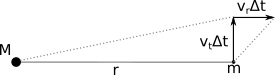
# So, now that we know that large bodies can be treated as if they were point masses, what can we derive from it? First let's consider two masses, $M$ and $m$, located at the positions below.
# 
# ![Setup](Figures/Cartesian_Polar_coords.png)
# 
# While the above has the x and y axes labelled, it's far more convenient to work in polar coordinates. Given that
# 
# \begin{align}
#     \hat{\textbf{r}} &= \cos \theta \hat{\textbf{i}} + \sin \theta \hat{\textbf{j}}\\
#     \hat{\pmb{\theta}} &= -\sin \theta \hat{\textbf{i}} + \cos \theta \hat{\textbf{j}}
# \end{align}
# 
# then we know
# 
# \begin{align}
#     \hat{\textbf{r}}\cdot\hat{\pmb{\theta}}&=0\\
#     \hat{\textbf{r}} \times \hat{\pmb{\theta}}&=\hat{\textbf{k}}
# \end{align}
# 
# From these definitions, we can derive the following time derivatives:
# 
# \begin{align}
#     \frac{ {\rm d} \hat{\textbf{r}} } { {\rm d} t} &= \hat{\pmb{\theta}} \frac{ {\rm d } \theta } { {\rm d } t }\\
#     \frac{ {\rm d} \hat{\pmb{\theta}} } { {\rm d} t} &= - \hat{\textbf{r}} \frac{ {\rm d } \theta } { {\rm d } t }
# \end{align}
# 
# The whole point of the above is that the velocity of the planet can then be written as
# 
# \begin{align}
#     \textbf{v} &= \frac{ {\rm d} \textbf{r}} { {\rm d} t} = \frac{ {\rm d} r } { {\rm d} t} \hat{\textbf{r}} + r \frac{ {\rm d} \hat{\textbf{r}} } { {\rm d} t}\\
#      &= v_r \hat{\textbf{r}} + v_t \hat{ \pmb{\theta}}
# \end{align}
# 
# The angular momentum of the planet is then
# $$
#     \textbf{L} = \textbf{r} \times \textbf{p}
# $$
# which, when you take the derivative with respect to time, gives
# $$
#     \frac{ {\rm d} \textbf{L} }{ {\rm d} t } = \frac{ {\rm d} \textbf{r}}{ {\rm d} t } \times \textbf{p} + \textbf{r} \times \frac{ {\rm d} \textbf{p}}{ {\rm d} t }
# $$
# using $\textbf{p}=m\textbf{v}$ and $\textbf{F}= m\frac{{\rm d} \textbf{v}}{{\rm d} t}$, we thus get
# $$
#     \frac{ {\rm d} \textbf{L} }{ {\rm d} t } = m (\textbf{v}\times\textbf{v})+\textbf{r}\times\textbf{F}
# $$
# The first term has to be 0 (a vector crossed with itself is 0) while for that last term must be zero as $\textbf{F}$ is parallel to $\textbf{r}$. Thus, for any central force
# $$
#     \frac{ {\rm d} \textbf{L}} {{\rm d} t} = 0
# $$
# 
# ## Kepler's Second Law
# So, if angular momentum is convered under gravity, what does that tell us about the orbit of (for example) a planet around a star? The angular momentum of the planet can be written as
# 
# \begin{align}
#     \textbf{L} &= \textbf{r} \times \textbf{p} \\
#     \textbf{L} &= m r v_t \hat{\textbf{k}}
# \end{align}
# 
# Now imagine a setup like that shown below, where we have a planet moving with a velocity $\textbf{v} = v_r \hat{\textbf{r}} + v_t \hat{ \pmb{\theta}}$. We're interested in how much area is swept out by the orbit of the planet in a time $\Delta t$.
# ![Planet_Vel](Figures/Planet_velocity.png)
# This is given by
# $$
#     \Delta A \approx \frac{1}{2} r v_t \Delta t + \frac{1}{2} r v_r \Delta t
# $$
# In the limit where $r>>v_r \Delta t$ (which is true for planets when considering very short timescales), we end up with
# $$
#     \Delta A \approx \frac{1}{2} r v_t \Delta t
# $$
# In the limit $t \to 0$ we then get
# $$
#     \lim_{t \to 0} \frac{\Delta A} {\Delta t} = \frac{{\rm d} A}{{\rm d} t} = \frac{1}{2} r v_t = \frac{L}{2 m}
# $$
# The important thing about this last term is that both $L$ and $m$ are constants, which means
# $$
#     \frac{{\rm d} A}{{\rm d} t} = {\rm constant}.
# $$
# This is Kepler's Second Law.
# 
# ## Kepler's First Law
# The above expressions can be used to state that
# $$
#     L = r^2 \frac{{\rm d} \theta}{{\rm d} t}
# $$
# which, following Kepler's Second Law, is constant for any central force. When that force is a gravitational force, we have that
# $$
#     \textbf{F} = -\frac{GMm}{r^2}\hat{\textbf{r}} = m\frac{{\rm d} \textbf{v}}{{\rm d}t }
# $$
# Following some simple math (Section 3.1.2 of Ryden & Peterson), we arrive at the following expression
# $$
#     r = \frac{L^2}{G M m^2 (1+e \cos \theta)}
# $$
# It can be shown that this expression can be written as
# $$
#     r = \frac{a(1-e^2)}{1+e \cos \theta}
# $$
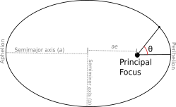
# where $a$ is the semimajor axis of the orbit, $e$ is the eccentricity of the orbit, and $\theta$ is called the "true anamoly".
# 
# ![Ellipse](Figures/Ellipse_Definitions.png)
# 
# As shown below, this is the equation for a conic section.
# 
# ![Conic_Sections](Figures/Conic_Sections.png)

# In[1]:


import numpy as np
import matplotlib.pyplot as plt

e = np.array([0.0,0.6,1.0,1.5])
# Polar coordinates
t = np.arange(-np.pi,np.pi,0.01)
theta = np.stack((t,) * 4, axis=-1)
r = (1-e**2)/(1+e*np.cos(theta))

#Cartesian coordinates
x = r.T*np.cos(theta.T)
y = r.T*np.sin(theta.T)

fig,ax = plt.subplots(nrows=1,ncols=1,figsize=[3.3,3], dpi=150)
#ax.plot(x[0],y[0], label='e=0, circular')
ax.plot(x[1],y[1], label='0<e<1, ellipse')
#ax.plot(x[2][np.where((t>-np.pi/1.4) & (t<np.pi/1.4))],y[2][np.where((t>-np.pi/1.4) & (t<np.pi/1.4))], label='e=1, parabola')
ax.plot(x[3][np.where((t>-np.pi/1.4) & (t<np.pi/1.4))],y[3][np.where((t>-np.pi/1.4) & (t<np.pi/1.4))], label='0<e<1, hyperbola')
ax.set_ylim(-3.12/2,3.12/2)
ax.set_xlim(-2.0,1.1)
ax.plot(0,0,'o',label='Focus')
#ax.plot(-1*e[3],0,'o',label='centre')
frame1 = plt.gca()
frame1.axes.get_xaxis().set_ticks([])
frame1.axes.get_yaxis().set_ticks([])
plt.legend(fontsize=5,loc=3)
plt.savefig("Figures/Orbits.svg")
plt.show()


# This expression allows for 4 types of orbits:
# 
# 1. A circular orbit ($e=0$).
# 2. An elliptical orbit ($0<e<1$).
# 3. A parabolic orbit ($e=1$).
# 4. A hyperbolic orbit ($e>1$).
# 
# As such, we've arrived at a generalisation of Kepler's First Law.
# 
# We can use the above expressions to determine what the velocity of the body throughout its orbit is by realising that
# $$
#     \frac{L^2}{m^2} = GMa(1-e^2)
# $$
# Knowing that $L=m v_t r$, we get
# $$
#     r^2 v_t^2 = GMa(1-e^2)
# $$
# Now, typically the velocity of the body is given by $\textbf{v} = v_r \hat{\textbf{r}} + v_t \hat{ \pmb{\theta}}$ - that is, there's both a radial and a tangential component. However, at perihelion, the velocity is entirely tangential, and we know that the distance between the planet and the Sun is $a(1-e)$. As such, at perihelion, the velocity is given by
# $$
#     v_{pe} = \left[\frac{GM}{a}\frac{1+e}{1-e}\right]^{1/2}
# $$
# A similar analysis at aphelion provides us with
# $$
#     v_{ap} = \left[\frac{GM}{a}\frac{1-e}{1+e}\right]^{1/2}
# $$

# In[ ]: