#!/usr/bin/env python
# coding: utf-8

# # 直连MICAPS Cassandra 数据库读取数值模式、卫星雷达等数据
# 
# #### —— nmc_met_io程序库读取MICAPS分布式数据环境（BDIPS）使用说明
# 
# 宜昌市气象局
# longtsing 2022，songofsongs@vip.qq.com
# 
# 
# MICAPS分布式数据环境（BDIPS）提供了两种访问方式:一种是直接连接读取Cassandra数据库，另外一种是基于Cassandra数据库上搭建的WEBService API方式检索读取。
# 
# [nmc_met_io](https://github.com/nmcdev/nmc_met_io)程序库的[retrieve_cassandraDB](https://github.com/nmcdev/nmc_met_io/blob/master/nmc_met_io/retrieve_micaps_server.py)模块, 基于Python Cassandra数据库接口包实现了Python语言对BDIPS数据的检索和读取。
# （注：由于WEBService的使用泛滥，各省已经限制该接口只能下载三天内的数据，为此启用Cassandra读取方式能延长读取数据的时效；但各省在Cassandra数据库存储数据时长也有不同，一般存储一周以上的数据。）
# 
# ### retrieve_cassandra模块主要功能:
# * 使用Cassandra的python接口, 读取程序库;
# * 接口定义与retrieve_micaps_server一致；
# * 引入的本地文件缓存技术, 加快数据的快速读取;
# * 支持模式数据标量场, 矢量场及集合成员数据的读取; 
# * 支持模式单点时间序列, 单点廓线及廓线时序的读取;
# * 支持站点, 探空观测数据的读取;
# * 支持awx格式的静止气象卫星等经纬度数据读取;
# * 支持LATLON格式的雷达拼图数据读取;
# * 统一的返回数据类型, 格点数据返回为[xarray](http://xarray.pydata.org/en/stable/)类型, 站点数据返回为[pandas.DataFrame](https://pandas.pydata.org/pandas-docs/stable/reference/api/pandas.DataFrame.html)类型.
# 
# ### 参考网站
# * https://github.com/nmcdev/nmc_met_io
# * https://github.com/datastax/python-driver
# * https://docs.datastax.com/en/developer/python-driver/3.25/getting_started/
# ---

# ## 1. 安装和配置nmc_met_io程序库
# 
# * 建议安装[Anaconda](https://www.anaconda.com/distribution/)的Python环境.
# * [nmc_met_io](https://github.com/nmcdev/nmc_met_io)有详细安装说明.
# * 需要配置Cassandra集群访问接口，具体在C:\Users\用户名\.nmcdev 目录下的config.ini内配置
# ```
# [Cassandra]
# ClusterIPAddresses=Cassandra集群IP地址以“,”分隔，可以参考MICAPS4的配置文件配置
# ClusterPort=Cassandra集群服务端口
# KeySpace=Cassandra上数据存储的主键名
# ```
# 

# In[1]:


# set up things
get_ipython().run_line_magic('matplotlib', 'inline')
get_ipython().run_line_magic('load_ext', 'autoreload')
get_ipython().run_line_magic('autoreload', '2')


# In[2]:


# load necessary libraries
# you should install cartopy with 'conda install -c conda-forge cartopy'
import xarray as xr
import numpy as np

# load nmc_met_io for retrieving micaps server data
import sys
sys.path.append("../nmc_met_io")
from retrieve_cassandraDB import *

xr.set_options(display_style="text")


# ## 2. 读取数值模式预报数据
# 
# 模块`retrieve_cassandraDB`提供读取数值模式网格预报数据的函数:
#  * `get_model_grid`: 读取单个时次标量, 矢量或集合成员的2D平面预报数据;
#  * `get_model_grids`: 读取多个时次标量, 矢量或集合成员的2D平面预报数据;
#  * `get_model_points`: 获取指定经纬度点的模式预报数据;
#  * `get_model_3D_grid`: 获得单个时次标量, 矢量或集合成员的[lev, lat, lon]3D预报数据;
#  * `get_model_3D_grids`: 获得多个时次标量, 矢量或集合成员的[lev, lat, lon]3D预报数据;
#  * `get_model_profiles`: 获得制定经纬度单点的模块廓线预报数据.
# 
# 每个函数都有固定的参数`directory`和`filename`(或`filenames`), 例如
# ```Python
# # MICAPS分布式服务器上的数据地址, 可通过MICAPS4的数据源检索界面查找,
# # 如下图, 找到数据存放的目录, 鼠标右键点击"保存路径到剪切板", 粘贴去掉"mdfs:///"
# directory = 'ECMWF_HR/TMP/850'
# # 指定具体的数据文件, 一般格式为"起报时间.预报时效", 若不指定, 则自动获得目录下最新数据的文件名
# filename = '22022408.024'
# # 调用函数读取数据
# data = get_model_grid(directory, filename=filename)
# ```
# 
# <img src="./images/micaps_retrieve_UI.png" alt="image" style="height: 400px;">

# ### 2.1 读取单个时次模式标量预报数据

# In[3]:


directory = 'ECMWF_HR/TMP/850'
filename = '22022408.024'
data = get_model_grid(directory, filename=filename, cache=False)
if data is not None:
    print(data)
else:
    print("Retrieve failed.")


# <div class="alert alert-success">
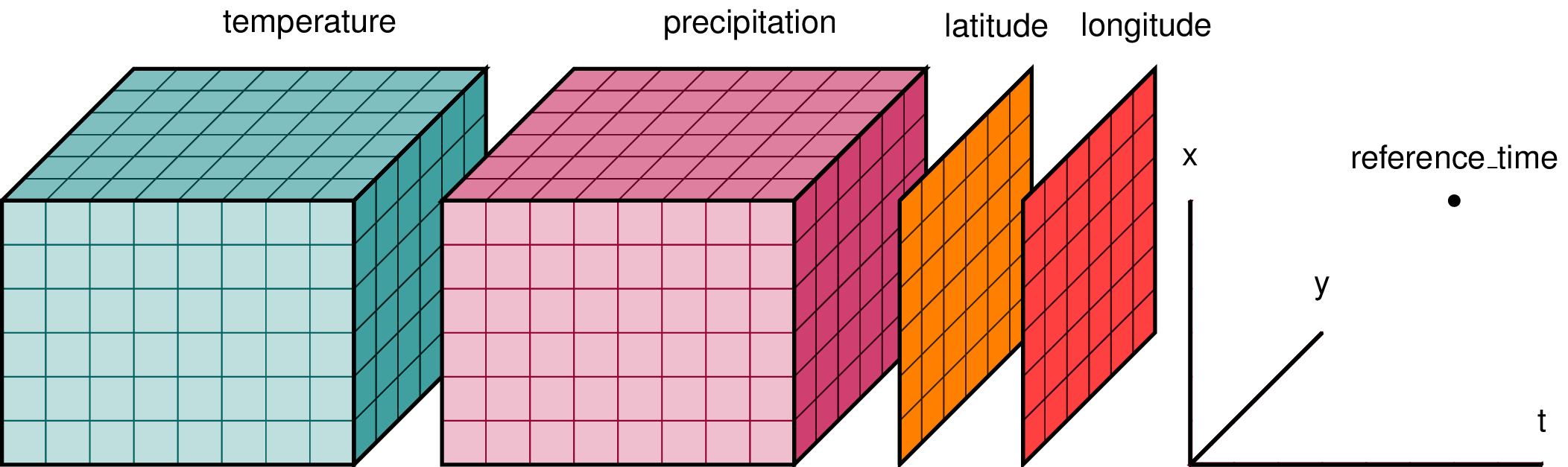
#     <b>返回xarray数据结构</b>:
#     <ul>
#         <li>返回的数据类型为[xarray](http://xarray.pydata.org/en/stable/)的Dataset结构数据(如下图所示).</li>
#         <li>xarray为在numpy数组基础上增加维度, 坐标和属性信息, 其数据模型来自于netCDF文件结构.</li>
#         <li>xarray提供直观,简介且可靠的格点数据操作功能, 已成为地球环境科学的标准数据处理程序库, 与很多现有的开源软件兼容.</li>
#         <li><em>get_model_grid</em>根据读取数据类型返回不同维度的Dataset数据. 如上对于高空数据, 返回数据的维度分别为(time, level, lat, lon).</li>
#         <li>在坐标Coordinate信息中, 除了数组维度的信息, 还给出起报时间forecast_reference_time和预报时效forecast_period</li>
#     </ul>
# </div>
# 
# <img src="./images/xarray_dataset.png" width="600">

# In[4]:


# 使用?可以获得函数的帮助信息.
get_ipython().run_line_magic('pinfo', 'get_model_grid')


# In[5]:


# 可以指定数据的变量名称, 变量属性等信息
data = get_model_grid(directory, filename=filename, varname='TEM', varattrs={'long_name':'temperature', 'units':'degree'}, cache=False)
if data is not None:
    print(data.TEM)
else:
    print("Retrieve failed.")


# In[6]:


import matplotlib as mpl  
import matplotlib.pyplot as plt
import cartopy.crs as ccrs


# In[7]:


# 绘制图像
fig = plt.figure(figsize=(12,8))
ax = plt.axes(projection=ccrs.LambertConformal(central_longitude=120))
data.TEM.plot(ax=ax, transform=ccrs.PlateCarree(), cbar_kwargs={'shrink': 0.8})
ax.coastlines()
ax.gridlines()
ax.set_extent([80,130,15,54], crs=ccrs.PlateCarree())


# ## 2.2 读取多个时次的模式预报数据

# In[8]:


get_ipython().run_line_magic('time', '')
directory = "ECMWF_HR/TMP/500"
fhours = np.arange(0, 132, 12)
filenames = ['22022208.'+'%03d'%(fhour) for fhour in fhours]
data = get_model_grids(directory, filenames, varname='HGT', varattrs={'long_name':'geopotential height', 'units':'dagpm'}, cache=False)


# In[9]:


data


# In[10]:


# 绘制图像
data.HGT.isel(level=0).plot.contour(col='time', col_wrap=4, levels=20)


# ## 2.3 读取集合预报数据

# In[11]:


get_ipython().run_line_magic('time', '')
directory = "ECMWF_ENSEMBLE/RAW/RAIN24"
filenames = get_file_list(directory)[:3]
data = get_model_grids(directory, filenames=filenames, varname='precipitation',
                      varattrs={'long_name':'accumulated precipitation', 'units':'mm'},
                      cache=False)
data


# In[13]:


# set colors and levels
clevs = [0.01, 2.5, 5, 10, 20, 40, 60]
colors = ['#b1f7a3', '#76d870', '#39bb3e', '#318c2f', '#5cb8fc', '#0202fd', '#ef08e9']
cmap, norm = mpl.colors.from_levels_and_colors(clevs, colors, extend='max')

plt.rcParams['font.size'] = '20'
subdata = data.sel(lon=slice(105, 110), lat=slice(29, 34))
fg = subdata.precipitation.isel(time=0).plot(
    col='number', col_wrap=8, cmap=cmap, norm=norm, extend="max", \
    sharex=True, sharey=True,
    cbar_kwargs={"aspect":40, "shrink":0.6, "pad":0.01})
fg.set_xlabels("Lon")
fg.set_ylabels("lat")


# ## 2.4 读取卫星图像数据

# In[14]:


# 获得风云4A中国区域4通道产品
directory = "SATELLITE/FY4A/L1/CHINA/C008"
data = get_fy_awx(directory)
data


# In[15]:


# 绘制图像
fig = plt.figure(figsize=(12,8))
ax = plt.axes(projection=ccrs.LambertConformal(central_longitude=100))
data.image[0,0,:,:].plot(ax=ax, transform=ccrs.PlateCarree(), cbar_kwargs={'shrink': 0.8})
ax.coastlines()
ax.gridlines()
ax.set_extent([80,130,15,54], crs=ccrs.PlateCarree())


# In[16]:


# 风云2静止卫星图像
directory = "SATELLITE/FY2/L1/IR1/EQUAL"
data = get_fy_awx(directory)

# 绘制图像
fig = plt.figure(figsize=(12,8))
ax = plt.axes(projection=ccrs.LambertConformal(central_longitude=100))
data.image[0,0,:,:].plot(ax=ax, transform=ccrs.PlateCarree(), cbar_kwargs={'shrink': 0.8}, cmap="gist_ncar", vmin=310, vmax=327)
ax.coastlines()
ax.gridlines()
ax.set_extent([80,130,15,54], crs=ccrs.PlateCarree())


# In[ ]: