#!/usr/bin/env python
# coding: utf-8
# This notebook is part of the `kikuchipy` documentation https://kikuchipy.org.
# Links to the documentation won't work from the notebook.
# # Reference frames
#
# ## Sample-detector geometry
#
# The figure below shows the [sample reference frame](#detector-sample-geometry)
# and the [detector reference frame](#detector-coordinates) used in kikuchipy, all
# of which are right handed. In short, the sample reference frame is the one used
# by EDAX TSL, RD-TD-ND, while the pattern center is defined as in the Bruker
# software.
#  # In **(a)** (lower left), a schematic of the microscope chamber shows the
# definition of the sample reference frame, RD-TD-ND. The
# $x_{euler}-y_{euler}-z_{euler}$ crystal reference frame used by Bruker is shown
# for reference. An EBSD pattern on the detector screen is viewed from *behind*
# the screen *towards* the sample. The inset **(b)** shows the detector and sample
# normals viewed from above, and the azimuthal angle $\omega$ which is defined as
# the sample tilt angle round the RD axis. **(c)** shows how the EBSD map appears
# within the data collection software, with the sample reference frame and the
# scanning reference frame, $x_{scan}-y_{scan}-z_{scan}$, attached. Note the
# $180^{\circ}$ rotation of the map about ND. **(d)** shows the relationship
# between the sample reference frame and the detector reference frame,
# $x_{detector}-y_{detector}-z_{detector}$, with the projection center
# highlighted. The detector tilt $\theta$ and sample tilt $\sigma$, in this case
# $10^{\circ}$ and $70^{\circ}$, respectively, are also shown.
#
# In **(a)** (lower left), a schematic of the microscope chamber shows the
# definition of the sample reference frame, RD-TD-ND. The
# $x_{euler}-y_{euler}-z_{euler}$ crystal reference frame used by Bruker is shown
# for reference. An EBSD pattern on the detector screen is viewed from *behind*
# the screen *towards* the sample. The inset **(b)** shows the detector and sample
# normals viewed from above, and the azimuthal angle $\omega$ which is defined as
# the sample tilt angle round the RD axis. **(c)** shows how the EBSD map appears
# within the data collection software, with the sample reference frame and the
# scanning reference frame, $x_{scan}-y_{scan}-z_{scan}$, attached. Note the
# $180^{\circ}$ rotation of the map about ND. **(d)** shows the relationship
# between the sample reference frame and the detector reference frame,
# $x_{detector}-y_{detector}-z_{detector}$, with the projection center
# highlighted. The detector tilt $\theta$ and sample tilt $\sigma$, in this case
# $10^{\circ}$ and $70^{\circ}$, respectively, are also shown.
# 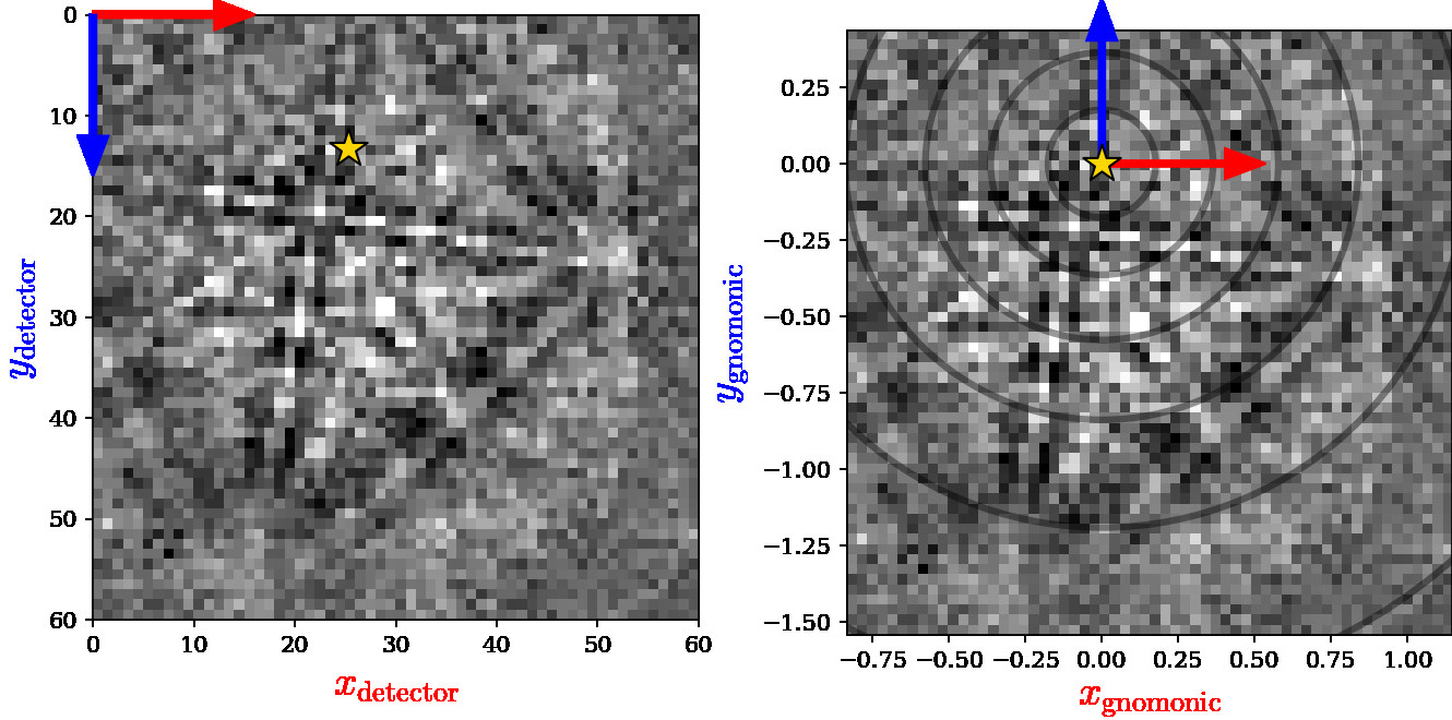 # The above figure shows the EBSD pattern in the
# [sample reference frame figure](#detector-sample-geometry) (a) as viewed from
# behind the screen towards the sample (left), with the detector reference frame
# the same as in (d) with its origin (0, 0) in the upper left pixel. The detector
# pixels' gnomonic coordinates can be described with a calibrated projection
# center (PC) (right), with the gnomonic reference frame origin (0, 0) in ($PC_x,
# PC_y$). The circles indicate the angular distance from the PC in steps of
# $10^{\circ}$.
# ## The EBSD detector
#
# All relevant parameters for the sample-detector geometry are stored in an
# [kikuchipy.detectors.EBSDDetector](../reference.rst#kikuchipy.detectors.EBSDDetector)
# instance. Let's first import necessary libraries and a small Nickel EBSD test
# data set
# In[ ]:
# Exchange inline for notebook or qt5 (from pyqt) for interactive plotting
get_ipython().run_line_magic('matplotlib', 'inline')
import matplotlib.pyplot as plt
import numpy as np
import kikuchipy as kp
s = kp.data.nickel_ebsd_small() # Use kp.load("data.h5") to load your own data
s
# Then we can define a detector with the same parameters as the one used to
# acquire the small Nickel data set
# In[ ]:
detector = kp.detectors.EBSDDetector(
shape=s.axes_manager.signal_shape[::-1],
pc=[0.421, 0.779, 0.505],
convention="tsl",
px_size=70, # microns
binning=8,
tilt=0,
sample_tilt=70
)
detector
# In[ ]:
detector.pc_tsl()
# The projection/pattern center (PC) is stored internally in the Bruker
# convention:
#
# - $PC_x$ is measured from the left border of the detector in fractions of detector
# width.
#
# - $PC_y$ is measured from the top border of the detector in fractions of detector
# height.
#
# - $PC_z$ is the distance from the detector scintillator to the sample divided by
# pattern height.
#
# Above, the PC was passed in the EDAX TSL convention. Passing the PC in the
# Bruker, Oxford, or EMsoft v4 or v5 convention is also supported. The definitions
# of the conventions are given in the
# [EBSDDetector](../reference.rst#kikuchipy.detectors.EBSDDetector) API reference,
# together with the conversion from PC coordinates in the TSL, Oxford, or EMsoft
# conventions to PC coordinates in the Bruker convention.
#
# The PC coordinates in the TSL, Oxford, or EMsoft conventions can be retreived
# via [EBSDDetector.pc_tsl()](../reference.rst#kikuchipy.detectors.EBSDDetector.pc_tsl),
# [EBSDDetector.pc_oxford()](../reference.rst#kikuchipy.detectors.EBSDDetector.pc_oxford),
# and [EBSDDetector.pc_emsoft()](../reference.rst#kikuchipy.detectors.EBSDDetector.pc_emsoft),
# respectively. The latter requires the unbinned detector pixel size in microns
# and the detector binning to be given upon initialization.
# In[ ]:
detector.pc_emsoft()
# The detector can be plotted to show whether the average PC is placed as
# expected using
# [EBSDDetector.plot()](../reference.rst#kikuchipy.detectors.EBSDDetector.plot) (see
# its docstring for a complete explanation of its parameters)
# In[ ]:
detector.plot(pattern=s.inav[0, 0].data)
# This will produce a figure similar to the left panel in the
# [detector coordinates figure](#detector-coordinates) above, without the arrows
# and colored labels.
#
# Multiple PCs with a 1D or 2D navigation shape can be passed to the `pc`
# parameter upon initialization, or can be set directly. This gives the detector
# a navigation shape (not to be confused with the detector shape) and a navigation
# dimension (maximum of two)
# In[ ]:
detector.pc = np.ones([3, 4, 3]) * [0.421, 0.779, 0.505]
detector.navigation_shape
# In[ ]:
detector.navigation_dimension
# In[ ]:
detector.pc = detector.pc[0, 0]
detector.navigation_shape
#
# The above figure shows the EBSD pattern in the
# [sample reference frame figure](#detector-sample-geometry) (a) as viewed from
# behind the screen towards the sample (left), with the detector reference frame
# the same as in (d) with its origin (0, 0) in the upper left pixel. The detector
# pixels' gnomonic coordinates can be described with a calibrated projection
# center (PC) (right), with the gnomonic reference frame origin (0, 0) in ($PC_x,
# PC_y$). The circles indicate the angular distance from the PC in steps of
# $10^{\circ}$.
# ## The EBSD detector
#
# All relevant parameters for the sample-detector geometry are stored in an
# [kikuchipy.detectors.EBSDDetector](../reference.rst#kikuchipy.detectors.EBSDDetector)
# instance. Let's first import necessary libraries and a small Nickel EBSD test
# data set
# In[ ]:
# Exchange inline for notebook or qt5 (from pyqt) for interactive plotting
get_ipython().run_line_magic('matplotlib', 'inline')
import matplotlib.pyplot as plt
import numpy as np
import kikuchipy as kp
s = kp.data.nickel_ebsd_small() # Use kp.load("data.h5") to load your own data
s
# Then we can define a detector with the same parameters as the one used to
# acquire the small Nickel data set
# In[ ]:
detector = kp.detectors.EBSDDetector(
shape=s.axes_manager.signal_shape[::-1],
pc=[0.421, 0.779, 0.505],
convention="tsl",
px_size=70, # microns
binning=8,
tilt=0,
sample_tilt=70
)
detector
# In[ ]:
detector.pc_tsl()
# The projection/pattern center (PC) is stored internally in the Bruker
# convention:
#
# - $PC_x$ is measured from the left border of the detector in fractions of detector
# width.
#
# - $PC_y$ is measured from the top border of the detector in fractions of detector
# height.
#
# - $PC_z$ is the distance from the detector scintillator to the sample divided by
# pattern height.
#
# Above, the PC was passed in the EDAX TSL convention. Passing the PC in the
# Bruker, Oxford, or EMsoft v4 or v5 convention is also supported. The definitions
# of the conventions are given in the
# [EBSDDetector](../reference.rst#kikuchipy.detectors.EBSDDetector) API reference,
# together with the conversion from PC coordinates in the TSL, Oxford, or EMsoft
# conventions to PC coordinates in the Bruker convention.
#
# The PC coordinates in the TSL, Oxford, or EMsoft conventions can be retreived
# via [EBSDDetector.pc_tsl()](../reference.rst#kikuchipy.detectors.EBSDDetector.pc_tsl),
# [EBSDDetector.pc_oxford()](../reference.rst#kikuchipy.detectors.EBSDDetector.pc_oxford),
# and [EBSDDetector.pc_emsoft()](../reference.rst#kikuchipy.detectors.EBSDDetector.pc_emsoft),
# respectively. The latter requires the unbinned detector pixel size in microns
# and the detector binning to be given upon initialization.
# In[ ]:
detector.pc_emsoft()
# The detector can be plotted to show whether the average PC is placed as
# expected using
# [EBSDDetector.plot()](../reference.rst#kikuchipy.detectors.EBSDDetector.plot) (see
# its docstring for a complete explanation of its parameters)
# In[ ]:
detector.plot(pattern=s.inav[0, 0].data)
# This will produce a figure similar to the left panel in the
# [detector coordinates figure](#detector-coordinates) above, without the arrows
# and colored labels.
#
# Multiple PCs with a 1D or 2D navigation shape can be passed to the `pc`
# parameter upon initialization, or can be set directly. This gives the detector
# a navigation shape (not to be confused with the detector shape) and a navigation
# dimension (maximum of two)
# In[ ]:
detector.pc = np.ones([3, 4, 3]) * [0.421, 0.779, 0.505]
detector.navigation_shape
# In[ ]:
detector.navigation_dimension
# In[ ]:
detector.pc = detector.pc[0, 0]
detector.navigation_shape
#
#
# Note
#
# The offset and scale of HyperSpy’s `axes_manager` is fixed for a signal,
# meaning that we cannot let the PC vary with scan position if we want to
# calibrate the EBSD detector via the `axes_manager`. The need for a varying
# PC was the main motivation behind the `EBSDDetector` class.
#
#
# The right panel in the [detector coordinates figure](#detector-coordinates)
# above shows the detector plotted in the gnomonic projection using
# [EBSDDetector.plot()](../reference.rst#kikuchipy.detectors.EBSDDetector.plot). We
# assign 2D gnomonic coordinates ($x_g, y_g$) in a gnomonic projection plane
# parallel to the detector screen to a 3D point ($x_d, y_d, z_d$) in the detector
# frame as
#
# $$
# x_g = \frac{x_d}{z_d}, \qquad y_g = \frac{y_d}{z_d}.
# $$
#
# The detector bounds and pixel scale in this projection, per navigation point,
# are stored with the detector
# In[ ]:
detector.bounds
# In[ ]:
detector.gnomonic_bounds
# In[ ]:
detector.x_range
# In[ ]:
detector.r_max # Largest radial distance to PC
# ## Projection center calibration
# The gnomonic projection (pattern) center (PC) of an EBSD detector can be
# estimated by the "moving-screen" technique
# Hjelen et al.. The technique relies
# on the assumption that the beam normal, shown in the
# [top figure (d)](#detector-sample-geometry) above, is normal to the detector
# screen as well as the incoming electron beam, and will therefore intersect the
# screen at a position independent of the detector distance (DD). To find this
# position, we need two EBSD patterns acquired with a stationary beam but with a
# known difference $\Delta z$ in DD, say 5 mm.
#
# First, the goal is to find the pattern position which does not shift between the
# two camera positions, ($PC_x$, $PC_y$). This point can be estimated in fractions
# of screen width and height, respectively, by selecting the same pattern features
# in both patterns. The two points of each pattern feature can then be used to
# form a straight line, and two or more such lines should intersect at ($PC_x$,
# $PC_y$).
#
# Second, the DD ($PC_z$) can be estimated from the same points. After finding
# the distances $L_{in}$ and $L_{out}$ between two points (features) in both
# patterns (in = operating position, out = 5 mm from operating position), the DD
# can be found from the relation
#
# $$
# \mathrm{DD} = \frac{\Delta z}{L_{out}/L_{in} - 1},
# $$
#
# where DD is given in the same unit as the known camera distance difference. If
# also the detector pixel size $\delta$ is known (e.g. 46 mm / 508 px), $PC_z$ can
# be given in the fraction of the detector screen height
#
# $$
# PC_z = \frac{\mathrm{DD}}{N_r \delta b},
# $$
#
# where $N_r$ is the number of detector rows and $b$ is the binning factor.
#
# Let's find an estimate of the PC from two single crystal Silicon EBSD patterns,
# which are included in the [kikuchipy.data](../reference.rst#data) module
# In[ ]:
s_in = kp.data.silicon_ebsd_moving_screen_in(allow_download=True)
s_in.remove_static_background()
s_in.remove_dynamic_background()
s_out5mm = kp.data.silicon_ebsd_moving_screen_out5mm(allow_download=True)
s_out5mm.remove_static_background()
s_out5mm.remove_dynamic_background()
# As a first approximation, we can find the detector pixel positions of the same
# features in both patterns by plotting them and noting the upper right
# coordianates provided by Matplotlib when plotting with an interactive backend
# (e.g. qt5 or notebook) and hovering over image pixels
# In[ ]:
fig, ax = plt.subplots(ncols=2, sharex=True, sharey=True, figsize=(20, 10))
ax[0].imshow(s_in.data, cmap="gray")
_ = ax[1].imshow(s_out5mm.data, cmap="gray")
# For this example we choose the positions of three zone axes. The PC calibration
# is performed by creating an instance of the
# [PCCalibrationMovingScreen](../reference.rst#kikuchipy.detectors.PCCalibrationMovingScreen)
# class
# In[ ]:
cal = kp.detectors.PCCalibrationMovingScreen(
pattern_in=s_in.data,
pattern_out=s_out5mm.data,
points_in=[(109, 131), (390, 139), (246, 232)],
points_out=[(77, 146), (424, 156), (246, 269)],
delta_z=5,
px_size=None, # Default
convention="tsl", # Default
)
cal
# We see that ($PC_x$, $PC_y$) = (0.5123, 0.8606), while DD = 21.7 mm. To get
# $PC_z$ in fractions of detector height, we have to provide the detector pixel
# size $\delta$ upon initialization, or set it directly and recalculate the PC
# In[ ]:
cal.px_size = 46 / 508 # mm/px
cal
# We can visualize the estimation by using the (opinionated) convenience method
# [PCCalibrationMovingScreen.plot()](../reference.rst#kikuchipy.detectors.PCCalibrationMovingScreen.plot)
# In[ ]:
cal.plot()
# As expected, the three lines in the right figure meet at a more or less the same
# position. We can replot the three images and zoom in on the PC to see how close
# they are to each other. We will use two standard deviations of all $PC_x$
# estimates as the axis limits (scaled with pattern shape)
# In[ ]:
# PCy defined from top to bottom, otherwise "tsl", defined from bottom to top
cal.convention = "bruker"
pcx, pcy, _ = cal.pc
two_std = 2 * np.std(cal.pcx_all, axis=0)
fig, ax = cal.plot(return_fig_ax=True)
ax[2].set_xlim([cal.ncols * (pcx - two_std), cal.ncols * (pcx + two_std)])
_ = ax[2].set_ylim([cal.nrows * ( pcy - two_std), cal.nrows * (pcy + two_std)])
# Finally, we can use this PC estimate along with the orientation of the Si
# crystal, as determined by Hough indexing with a commercial software, to see how
# good the estimate is, by performing a
# [geometrical EBSD simulation](geometrical_ebsd_simulations.ipynb) of positions of
# Kikuchi band centres and zone axes from the five $\{hkl\}$ families $\{111\}$,
# $\{200\}$, $\{220\}$, $\{222\}$, and $\{311\}$
# In[ ]:
from diffsims.crystallography import ReciprocalLatticePoint
from orix import crystal_map, quaternion
# Create simulation generator from a detector and crystal phase and orientation
detector = kp.detectors.EBSDDetector(
shape=cal.shape, pc=cal.pc, sample_tilt=70, convention=cal.convention
)
phase = crystal_map.Phase(space_group=227)
r = quaternion.Rotation.from_euler(np.deg2rad([133.3, 88.7, 177.8]))
simgen = kp.generators.EBSDSimulationGenerator(
detector=detector, phase=phase, rotations=r
)
simgen.navigation_shape = s_in.axes_manager.navigation_shape
# Specify which plane families for which to simulate bands and zone axes
rlp = ReciprocalLatticePoint(
phase=phase, hkl=[[1, 1, 1], [2, 0, 0], [2, 2, 0], [2, 2, 2], [3, 1, 1]]
).symmetrise() # Symmetrise to get all symmetrically equivalent planes
simgeo = simgen.geometrical_simulation(rlp)
#del s_in.metadata.Markers # Uncomment this if we want to re-add markers
s_in.add_marker(
marker=simgeo.as_markers(),
plot_marker=False,
permanent=True
)
s_in.plot(navigator=None, colorbar=False, axes_off=True, title="")
# The PC is not perfect, but the estimate might be good enough for a further PC
# and/or orientation refinement.