#!/usr/bin/env python
# coding: utf-8
# OpenSees Examples Manual Examples for OpenSeesPy
# OpenSees Example 9. Build & Analyze a Section Example
#
#
#
# You can find the original Examples:
# https://opensees.berkeley.edu/wiki/index.php/Examples_Manual
# Original Examples by By Silvia Mazzoni & Frank McKenna, 2006, in Tcl
# Converted to OpenSeesPy by SilviaMazzoni, 2020
# This Example:
# https://opensees.berkeley.edu/wiki/index.php/OpenSees_Example_9._Build_%26_Analyze_a_Section_Example
#
#
# This workbook demonstrates a Moment-Curvature analysis for two types of sections
# 1. A uniaxial Section (moment-curvature relationship).
# For the case of the uniaxial section, moment-curvature and axial force-deformation curves are defined independently, and numerically. The uniaxialMaterial command is used to define the moment-curvature relationship.
# 2. A fiber section (standard W section).
# For the case of the fiber sections (steel and RC), uniaxial materials are defined numerically (stress-strain relationship) and are combined into a fiber section where moment-curvature and axial force-deformation characteristics and their interaction are calculated computationally.
#
# Even though the sections are defined differently, the process of computing the moment-curvature response are the same, as demonstrated in this example.
#
# For more info on Fiber Recorders, visit the Portwood Digital blog on this topic here
#
#
#
#
2D vs. 3D
# While this distinction does not affect the section definition itself, it affects the degree-of-freedom associated with moment and curvature in the subsequent analysis.
# There are two differences between the two models:
#
# - The space defined with the model command (# Define the model builder, ndm=#dimension, ndf=#dofs)
# - 2D: model BasicBuilder -ndm 2 -ndf 3;
# - 3D: model BasicBuilder -ndm 3 -ndf 6;
# - In the 3D model, torsional stiffness needs to be aggregated to the section
#
# This example demonstrates the case of 2D
#
#
#
# Objectives of Example
# - Build a uniaxialSection: Flexure and axial behavior are uncoupled in this type of section
# - Perform a moment-curvature analysis on Section
#
#
#
# uniaxial Section:
# 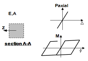 #
# |
# Fiber Section:
#  #
# |
#
#
#
#
# In[1]:
############################################################
# EXAMPLE:
# pyEx9a.build.UniaxialSection2D.tcl.py
# for OpenSeesPy
# --------------------------------------------------------#
# by: Silvia Mazzoni, 2020
# silviamazzoni@yahoo.com
############################################################
# This file was obtained from a conversion of the updated Tcl script
# The Tcl script was obtained by updating the Examples Manual published in the OpenSees Wiki Page
############################################################
import openseespy.opensees as ops
import os
import math
import eSEESminiPy
import numpy as numpy
import matplotlib.pyplot as plt
# --------------------------------------------------------------------------------------------------
# build a section
# Silvia Mazzoni and Frank McKenna, 2006
#
# SET UP ----------------------------------------------------------------------------
dataDir = 'Data' # set up name of data directory -- simple
if not os.path.exists(dataDir):
os.mkdir(dataDir)
# --------------------------------------------------------------------------------------------------
# LibUnits.tcl -- define system of units
# Silvia Mazzoni and Frank McKenna, 2006
#
# define UNITS ----------------------------------------------------------------------------
inch = 1. # define basic units -- output units
kip = 1. # define basic units -- output units
sec = 1. # define basic units -- output units
LunitTXT = 'inch' # define basic-unit text for output
FunitTXT = 'kip' # define basic-unit text for output
TunitTXT = 'sec' # define basic-unit text for output
ft = 12.*inch # define engineering units
ksi = kip/math.pow(inch,2)
psi = ksi/1000.
lbf = psi*inch*inch # pounds force
pcf = lbf/math.pow(ft,3) # pounds per cubic foot
psf = lbf/math.pow(ft,3) # pounds per square foot
inch2 = inch*inch # inch^2
inch4 = inch*inch*inch*inch # inch^4
cm = inch/2.54 # centimeter, needed for displacement input in MultipleSupport excitation
PI = 2*math.asin(1.0) # define constants
g = 32.2*ft/math.pow(sec,2) # gravitational acceleration
Ubig = 1.e10 # a really large number
Usmall = 1/Ubig # a really small number
# In[2]:
# Define a function to run moment-curvature analysis
############################################################
# EXAMPLE:
# pyLibMomentCurvature2D.tcl.py
# for OpenSeesPy
# --------------------------------------------------------#
# by: Silvia Mazzoni, 2020
# silviamazzoni@yahoo.com
############################################################
# This file was obtained from a conversion of the updated Tcl script
# The Tcl script was obtained by updating the Examples Manual published in the OpenSees Wiki Page
############################################################
def MomentCurvature2D(secTag,axialLoad,maxK,numIncr,fiberRecorderData={}):
##################################################
# A procedure for performing section analysis (only does
# moment-curvature, but can be easily modified to do any mode
# of section reponse.)
#
# MHS
# October 2000
# modified to 2D and to improve convergence by Silvia Mazzoni, 2006
# converted to OpenSeesPy by Silvia Mazzoni, 2020
#
# Arguments
# secTag -- tag identifying section to be analyzed
# axialLoad -- axial load applied to section (negative is compression)
# maxK -- maximum curvature reached during analysis
# numIncr -- number of increments used to reach maxK (default 100)
#
# Sets up a recorder which writes moment-curvature results to file
# sectionsecTag.out ... the moment is in column 1, and curvature in column 2
# Define two nodes at (0,0)
ops.node(1001,0.0,0.0)
ops.node(1002,0.0,0.0)
# Fix all degrees of freedom except axial and bending
ops.fix(1001,1,1,1)
ops.fix(1002,0,1,0)
# Define element
# tag ndI ndJ secTag
ops.element('zeroLengthSection',2001,1001,1002,secTag)
# Create recorder
ops.recorder('Node','-file','Mphi.out','-time','-node',1002,'-dof',3,'disp') # output moment (col 1) and curvature (col 2)
for thisLabel,thisData in fiberRecorderData.items():
print(thisData)
ops.recorder('Element','-ele',2001,'-file','FiberResponse_'+thisLabel+'.out','section','fiber',*thisData,'stressStrain') # output moment (col 1) and curvature (col 2)
# Define constant axial load
ops.timeSeries('Constant',3001) # timeSeries Constant 3001;
# define Load Pattern
ops.pattern('Plain',3001,3001) #
ops.load(1002,axialLoad,0.0,0.0)
# Define analysis parameters
ops.wipeAnalysis() # adding this to clear Analysis module
ops.constraints('Plain')
ops.integrator('LoadControl',0,1,0,0)
ops.system('SparseGeneral','-piv') # Overkill, but may need the pivoting!
ops.test('EnergyIncr',1.0e-9,10)
ops.numberer('Plain')
ops.algorithm('Newton')
ops.analysis('Static')
# Do one analysis for constant axial load
ops.analyze(1)
ops.loadConst('-time',0.0)
# Define reference moment
ops.timeSeries('Linear',3002) # timeSeries Linear 3002;
# define Load Pattern
ops.pattern('Plain',3002,3002) #
ops.load(1002,0.0,0.0,1.0)
# Compute curvature increment
dK = maxK/numIncr
# Use displacement control at node 1002 for section analysis, dof 3
ops.integrator('DisplacementControl',1002,3,dK,1,dK,dK)
# Do the section analysis
ok = ops.analyze(numIncr)
# ----------------------------------------------if convergence failure-------------------------
IDctrlNode = 1002
IDctrlDOF = 3
Dmax = 'maxK'
Dincr = dK
TolStatic = 1.e-9
testTypeStatic = 'EnergyIncr'
maxNumIterStatic = 6
algorithmTypeStatic = 'Newton'
#fmt1 = [%s,Pushover,analysis:,CtrlNode,%.3i,dof,%.1i,Curv=%.4f,/%s] # format for screen/file output of DONE/PROBLEM analysis
global LunitTXT ##xx## # load time-unit text
if ok != 0 :
# if analysis fails, we try some other stuff, performance is slower inside this loop
Dstep = 0.0
ok = 0
while Dstep <= 1.0 and ok == 0 :
controlDisp = ops.nodeDisp(IDctrlNode,IDctrlDOF)
Dstep = controlDisp/Dmax
ok = ops.analyze(1) # this will return zero if no convergence problems were encountered
if ok != 0 :
Nk = 4 # reduce step size
DincrReduced = Dincr/Nk
ops.integrator('DisplacementControl',IDctrlNode,IDctrlDOF,DincrReduced)
for ik in range(1,Nk+1,1):
ok = ops.analyze(1) # this will return zero if no convergence problems were encountered
if ok != 0 :
# if analysis fails, we try some other stuff
# performance is slower inside this loop global maxNumIterStatic ##xx## # max no. of iterations performed before "failure to converge" is ret'd
print(' "Trying Newton with Initial Tangent ..')
ops.test('NormDispIncr',TolStatic,2000,0)
ops.algorithm('Newton','-initial')
ok = ops.analyze(1)
ops.test(testTypeStatic,TolStatic,maxNumIterStatic,0)
ops.algorithm(algorithmTypeStatic)
if ok != 0 :
print(' "Trying Broyden ..')
ops.algorithm('Broyden',8)
ok = ops.analyze(1)
ops.algorithm(algorithmTypeStatic)
if ok != 0 :
print(' "Trying NewtonWithLineSearch ..')
ops.algorithm('NewtonLineSearch',0.8)
ok = ops.analyze(1)
ops.algorithm(algorithmTypeStatic)
if ok != 0 :
print('PROBLEM')
return
ops.integrator('DisplacementControl',IDctrlNode,IDctrlDOF,Dincr) # bring back to original increment
# -----------------------------------------------------------------------------------------------------
if ok != 0 :
print('PROBLEM at NodeDisp=' + str(ops.nodeDisp(IDctrlNode,IDctrlDOF)) + LunitTXT)
else :
print('DONE! at NodeDisp=' + str(ops.nodeDisp(IDctrlNode,IDctrlDOF)) + LunitTXT)
# In[3]:
# UNIAXIAL SECTION IN 2d
ops.wipe() # clear memory of all past model definitions
ops.model('BasicBuilder','-ndm',2,'-ndf',3) # Define the model builder, ndm= dimension, ndf= dofs
# Define your SECTION
# MATERIAL parameters -------------------------------------------------------------------
SecTagFlex = 2 # assign a tag number to the column flexural behavior
SecTagAxial = 3 # assign a tag number to the column axial behavior
SecTag = 1 # assign a tag number to the column section tag
# COLUMN section
# calculated stiffness parameters
EASec = Ubig # assign large value to axial stiffness
MySec = 130000*kip*inch # yield moment
PhiYSec = 0.65e-4/inch # yield curvature
EICrack = MySec/PhiYSec # cracked section inertia
b = 0.01 # strain-hardening ratio (ratio between post-yield tangent and initial elastic tangent)
ops.uniaxialMaterial('Steel01',SecTagFlex,MySec,EICrack,b) # bilinear behavior for flexural moment-curvature
ops.uniaxialMaterial('Elastic',SecTagAxial,EASec) # this is not used as a material, this is an axial-force-strain response
ops.section('Aggregator',SecTag,SecTagAxial,'P',SecTagFlex,'Mz') # combine axial and flexural behavior into one section (no P-M interaction here)
# In[4]:
# Perform Moment-Curvature Analysis
# set AXIAL LOAD --------------------------------------------------------
P = -1800*kip #+Tension,-Compression
# set maximum Curvature:
Ku = 0.01/inch
numIncr = 1000 # Number of analysis increments to maximum curvature (default=100)
# Call the section analysis procedure
MomentCurvature2D(SecTag,P,Ku,numIncr)
ops.wipe()
fname3 = 'Mphi.out'
dataDFree = numpy.loadtxt(fname3)
plt.plot(dataDFree[:,1],dataDFree[:,0])
plt.ylabel('Pseudo-Time (~Moment)')
plt.xlabel('Curvature')
plt.title('Ex9.analyze.MomentCurvature2D.tcl')
plt.grid(True)
plt.show()
# In[5]:
# FIBER SECTION IN 2D
# Steel W Section
# SET UP ----------------------------------------------------------------------------
ops.wipe() # clear memory of all past model definitions
ops.model('BasicBuilder','-ndm',2,'-ndf',3) # Define the model builder, ndm= dimension, ndf= dofs
# MATERIAL parameters -------------------------------------------------------------------
# define MATERIAL properties ----------------------------------------
Fy = 60.0*ksi
Es = 29000*ksi # Steel Young's Modulus
nu = 0.3
Gs = Es/2./(1+nu) # Torsional stiffness Modulus
Hiso = 0
Hkin = 1000
matIDhard = 1
ops.uniaxialMaterial('Hardening',matIDhard,Es,Fy,Hiso,Hkin)
# Structural-Steel W-section properties -------------------------------------------------------------------
SecTag = 1
WSec = 'W27x114'
# from Steel Manuals:
# in × lb/ft Area (in2) d (in) bf (in) tf (in) tw (in) Ixx (in4) Iyy (in4)
# W27x114 33.5 27.29 10.07 0.93 0.57 4090 159
d = 27.29*inch # nominal depth
tw = 0.57*inch # web thickness
bf = 10.07*inch # flange width
tf = 0.93*inch # flange thickness
nfdw = 16 # number of fibers along web depth
nftw = 4 # number of fibers along web thickness
nfbf = 16 # number of fibers along flange width (you want this many in a bi-directional loading)
nftf = 4 # number of fibers along flange thickness
dw = d-2 * tf
y1 = -d/2
y2 = -dw/2
y3 = dw/2
y4 = d/2
z1 = -bf/2
z2 = -tw/2
z3 = tw/2
z4 = bf/2
#
# define Section
ops.section('Fiber',SecTag,'-GJ',1e9) #
# nfIJ nfJK yI zI yJ zJ yK zK yL zL
ops.patch('quadr',matIDhard,nfbf,nftf,y1,z4,y1,z1,y2,z1,y2,z4)
ops.patch('quadr',matIDhard,nftw,nfdw,y2,z3,y2,z2,y3,z2,y3,z3)
ops.patch('quadr',matIDhard,nfbf,nftf,y3,z4,y3,z1,y4,z1,y4,z4)
fiberRecorderData = {}
fiberRecorderData['topCtr'] = [y4,0.] # no need for a material tag since there is only one material
fiberRecorderData['origin'] = [0.,0.]
fiberRecorderData['botCtr'] = [y1,0.]
fiberRecorderData['topLeft'] = [y4,z4] # no need for a material tag since there is only one material
fiberRecorderData['botLeft'] = [y1,z4]
fiberRecorderData['topRight'] = [y4,z1] # no need for a material tag since there is only one material
fiberRecorderData['botRight'] = [y1,z1]
# In[6]:
# PERFORM ANALYSIS.
# This block of commands is the same as above
# Perform Moment-Curvature Analysis
# set AXIAL LOAD --------------------------------------------------------
P = -1800*kip #+Tension,-Compression
P = 0*kip #+Tension,-Compression
# set maximum Curvature:
Ku = 0.01/inch
numIncr = 1000 # Number of analysis increments to maximum curvature (default=100)
# Call the section analysis procedure
MomentCurvature2D(SecTag,P,Ku,numIncr,fiberRecorderData)
ops.wipe()
fname3 = 'Mphi.out'
dataDFree = numpy.loadtxt(fname3)
plt.plot(dataDFree[:,1],dataDFree[:,0])
plt.xlabel('Curvature')
plt.ylabel('Pseudo-Time (~Moment)')
plt.title('Ex9.analyze.MomentCurvature2D.tcl')
plt.grid(True)
plt.show()
# In[7]:
# look at fiber response:
for thisLabel,thisData in fiberRecorderData.items():
fname3 = 'FiberResponse_'+thisLabel+'.out'
dataDFree = numpy.loadtxt(fname3)
plt.plot(dataDFree[:,1],dataDFree[:,0])
plt.xlabel('Strain')
plt.ylabel('Stress')
plt.title('Fiber Response:' + thisLabel)
plt.grid(True)
plt.show()
# In[ ]: