 #
#
#
#
#  #
#
 # You can use multiple different kernels. The number of output channels corresponds to the number of kernel you use.
#
# You can use multiple different kernels. The number of output channels corresponds to the number of kernel you use.
#  # ## Trying on a real image
# In[ ]:
from PIL import Image
image = Image.open("image-city.jpg")
print(image.size)
image
# #### **Your Turn !**
# **Fill in the code cell below to perform the convolution of the above image with a kernel.**
# We will use a boundary detector filter as kernel:
#
# $$\begin{bmatrix}
# -1 & 0 & 1 \\
# -1 & 0 & 1 \\
# -1 & 0 & 1
# \end{bmatrix}
# $$
#
# Pay attention to the dimensions of the input and the kernel:
# - Input Size: **Batch size** x **Num channels** x **Input height** x **Input width**
# - Kernel Size: **Num output channels** x **Num input channels** x **Kernel height** x **Kernel width**
#
# Note:
# - There are 3 input channels (since we have an rgb image)
# - In output, we want only one channel (ie. we define only one kernel)
# - Here, batch size will be 1.
# In[ ]:
# %load -r 1-8 solutions/solution_5.py
from torchvision.transforms.functional import to_tensor, to_pil_image
image_tensor = to_tensor(image)
input = image_tensor.unsqueeze(0)
kernel = torch.Tensor([-1,0,1]).expand(1,3,3,3)
out = torch.nn.functional.conv2d(input, kernel)
# In[ ]:
norm_out = (out - out.min()) / (out.max() - out.min()) # Map output to [0,1] for visualisation purposes
to_pil_image(norm_out.squeeze())
# ## Convolutions in `nn.Module`
#
# When using a convolution layer inside an `nn.Module`, we rather use the `nn.Conv2d` module.
# The kernels of the convolution are directly instantiated by `nn.Conv2d`.
# In[ ]:
conv_1 = nn.Conv2d(in_channels=3, out_channels=2, kernel_size=(3,3))
print("Convolution", conv_1)
print("Kernel size: ", conv_1.weight.shape) # First two dimensions are: Num output channels and Num input channels
# In[ ]:
# Fake 5x5 input with 3 channels
input = torch.randn(1, 3, 5, 5) # batch_size, num_channels, height, width
out = conv_1(input)
print(out)
# _Animations credits: Francois Fleuret, Vincent Dumoulin_
# ---
# # Building a CNN
# We will use the MNIST classification dataset again as our learning task. However, this time we will try to solve it using Convolutional Neural Networks. Let's build the LeNet-5 CNN with PyTorch !
# ## Defining the LeNet-5 architecture
# 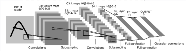
# *Y. LeCun, L. Bottou, Y. Bengio, and P. Haffner. "Gradient-based learning applied to document recognition." Proceedings of the IEEE, 86(11):2278-2324, November 1998.*
# _Note: The *Gaussian connections* in the last layer were used to estimate the lack of fit. In our implementation, we use a cross-entropy loss function as it's common nowadays. Similarly, ReLU are used instead of tanh activation._
#
# **Architecture Details**
#
# + Convolutional part:
#
#
# | Layer | Name | Input channels | Output channels | Kernel | stride |
# | ----------- | :--: | :------------: | :-------------: | :----: | :----: |
# | Convolution | C1 | 1 | 6 | 5x5 | 1 |
# | ReLU | | 6 | 6 | | |
# | MaxPooling | S2 | 6 | 6 | 2x2 | 2 |
# | Convolution | C3 | 6 | 16 | 5x5 | 1 |
# | ReLU | | 16 | 16 | | |
# | MaxPooling | S4 | 16 | 16 | 2x2 | 2 |
# | Convolution | C5 | 16 | 120 | 5x5 | 1 |
# | ReLU | | 120 | 120 | | |
#
#
# + Fully Connected part:
#
# | Layer | Name | Input size | Output size |
# | ---------- | :--: | :--------: | :---------: |
# | Linear | F5 | 120 | 84 |
# | ReLU | | | |
# | Linear | F6 | 84 | 10 |
# | LogSoftmax | | | |
#
# #### **Your turn !**
# Write a Pytorch module for the LeNet-5 model.
# You may need to use : `nn.Sequential`, `nn.Conv2d`, `nn.ReLU`, `nn.MaxPool2d`, `nn.Linear`, `nn.LogSoftmax`, `nn.Flatten`
# In[ ]:
# %load -s LeNet5 solutions/solution_5.py
class LeNet5(nn.Module):
def __init__(self):
super(LeNet5, self).__init__()
# YOUR TURN
def forward(self, imgs):
# YOUR TURN
return output
# An extensive list of all available layer types can be found on https://pytorch.org/docs/stable/nn.html.
# ### Print a network summary
# In[ ]:
conv_net = LeNet5()
print(conv_net)
# ### Retrieve trainable parameters
# In[ ]:
named_params = list(conv_net.named_parameters())
print("len(params): %s\n" % len(named_params))
for name, param in named_params:
print("%s:\t%s" % (name, param.shape))
# ### Feed network with a random input
# In[ ]:
input = torch.randn(1, 1, 32, 32) # batch_size, num_channels, height, width
out = conv_net(input)
print("Log-Probabilities: \n%s\n" % out)
print("Probabilities: \n%s\n" % torch.exp(out))
print("out.shape: \n%s" % (out.shape,))
# ---
# # Training our CNN
# ### Train function
#
# Similarly to the previous notebook, we define a train function `train_cnn`.
# In[ ]:
def train_cnn(model, train_loader, test_loader, device, num_epochs=3, lr=0.1):
# define an optimizer and a loss function
optimizer = torch.optim.Adam(model.parameters(), lr=lr)
criterion = torch.nn.CrossEntropyLoss()
for epoch in range(num_epochs):
print("=" * 40, "Starting epoch %d" % (epoch + 1), "=" * 40)
model.train() # Not necessary in our example, but still good practice.
# Only models with nn.Dropout and nn.BatchNorm modules require it
# dataloader returns batches of images for 'data' and a tensor with their respective labels in 'labels'
for batch_idx, (data, labels) in enumerate(train_loader):
data, labels = data.to(device), labels.to(device)
optimizer.zero_grad()
output = model(data)
loss = criterion(output, labels)
loss.backward()
optimizer.step()
if batch_idx % 40 == 0:
print("Batch %d/%d, Loss=%.4f" % (batch_idx, len(train_loader), loss.item()))
# Compute the train and test accuracy at the end of each epoch
train_acc = accuracy(model, train_loader, device)
test_acc = accuracy(model, test_loader, device)
print(colorama.Fore.GREEN, "\nAccuracy on training: %.2f%%" % (100*train_acc))
print("Accuracy on test: %.2f%%" % (100*test_acc), colorama.Fore.RESET)
# ### Test function
# We also define an `accuracy` function which can evaluate our model's accuracy on train/test data
# In[ ]:
def accuracy(model, dataloader, device):
""" Computes the model's accuracy on the data provided by 'dataloader'
"""
model.eval()
num_correct = 0
num_samples = 0
with torch.no_grad(): # deactivates autograd, reduces memory usage and speeds up computations
for data, labels in dataloader:
data, labels = data.to(device), labels.to(device)
predictions = model(data).max(1)[1] # indices of the maxima along the second dimension
num_correct += (predictions == labels).sum().item()
num_samples += predictions.shape[0]
return num_correct / num_samples
# ### Loading the train and test data with *`dataloaders`*
# In[ ]:
from torchvision import datasets, transforms
transformations = transforms.Compose([
transforms.Resize((32, 32)),
transforms.ToTensor()
])
train_data = datasets.MNIST('./data',
train = True,
download = True,
transform = transformations)
test_data = datasets.MNIST('./data',
train = False,
download = True,
transform = transformations)
train_loader = torch.utils.data.DataLoader(train_data, batch_size=256, shuffle=True)
test_loader = torch.utils.data.DataLoader(test_data, batch_size=1024, shuffle=False)
# ### Start the training!
# In[ ]:
device = torch.device('cuda' if torch.cuda.is_available() else 'cpu')
conv_net.to(device)
train_cnn(conv_net, train_loader, test_loader, device, lr=2e-3)
# ### Let's look at some of the model's predictions
# In[ ]:
def visualize_predictions(model, dataloader, device):
data, labels = next(iter(dataloader))
data, labels = data[:10].to(device), labels[:10]
predictions = model(data).max(1)[1]
predictions, data = predictions.cpu(), data.cpu()
plt.figure(figsize=(16,9))
for i in range(10):
img = data.squeeze(1)[i]
plt.subplot(1, 10, i+1)
plt.imshow(img, cmap="gray", interpolation="none")
plt.xlabel(predictions[i].item(), fontsize=18)
plt.xticks([])
plt.yticks([])
visualize_predictions(conv_net, test_loader, device)
# ___
#
# # < [Modules](5-Modules.ipynb) | Convolutional Neural Networks | [Transfer Learning](7-Transfer-Learning.ipynb) >
#
#
# ## Trying on a real image
# In[ ]:
from PIL import Image
image = Image.open("image-city.jpg")
print(image.size)
image
# #### **Your Turn !**
# **Fill in the code cell below to perform the convolution of the above image with a kernel.**
# We will use a boundary detector filter as kernel:
#
# $$\begin{bmatrix}
# -1 & 0 & 1 \\
# -1 & 0 & 1 \\
# -1 & 0 & 1
# \end{bmatrix}
# $$
#
# Pay attention to the dimensions of the input and the kernel:
# - Input Size: **Batch size** x **Num channels** x **Input height** x **Input width**
# - Kernel Size: **Num output channels** x **Num input channels** x **Kernel height** x **Kernel width**
#
# Note:
# - There are 3 input channels (since we have an rgb image)
# - In output, we want only one channel (ie. we define only one kernel)
# - Here, batch size will be 1.
# In[ ]:
# %load -r 1-8 solutions/solution_5.py
from torchvision.transforms.functional import to_tensor, to_pil_image
image_tensor = to_tensor(image)
input = image_tensor.unsqueeze(0)
kernel = torch.Tensor([-1,0,1]).expand(1,3,3,3)
out = torch.nn.functional.conv2d(input, kernel)
# In[ ]:
norm_out = (out - out.min()) / (out.max() - out.min()) # Map output to [0,1] for visualisation purposes
to_pil_image(norm_out.squeeze())
# ## Convolutions in `nn.Module`
#
# When using a convolution layer inside an `nn.Module`, we rather use the `nn.Conv2d` module.
# The kernels of the convolution are directly instantiated by `nn.Conv2d`.
# In[ ]:
conv_1 = nn.Conv2d(in_channels=3, out_channels=2, kernel_size=(3,3))
print("Convolution", conv_1)
print("Kernel size: ", conv_1.weight.shape) # First two dimensions are: Num output channels and Num input channels
# In[ ]:
# Fake 5x5 input with 3 channels
input = torch.randn(1, 3, 5, 5) # batch_size, num_channels, height, width
out = conv_1(input)
print(out)
# _Animations credits: Francois Fleuret, Vincent Dumoulin_
# ---
# # Building a CNN
# We will use the MNIST classification dataset again as our learning task. However, this time we will try to solve it using Convolutional Neural Networks. Let's build the LeNet-5 CNN with PyTorch !
# ## Defining the LeNet-5 architecture
# 
# *Y. LeCun, L. Bottou, Y. Bengio, and P. Haffner. "Gradient-based learning applied to document recognition." Proceedings of the IEEE, 86(11):2278-2324, November 1998.*
# _Note: The *Gaussian connections* in the last layer were used to estimate the lack of fit. In our implementation, we use a cross-entropy loss function as it's common nowadays. Similarly, ReLU are used instead of tanh activation._
#
# **Architecture Details**
#
# + Convolutional part:
#
#
# | Layer | Name | Input channels | Output channels | Kernel | stride |
# | ----------- | :--: | :------------: | :-------------: | :----: | :----: |
# | Convolution | C1 | 1 | 6 | 5x5 | 1 |
# | ReLU | | 6 | 6 | | |
# | MaxPooling | S2 | 6 | 6 | 2x2 | 2 |
# | Convolution | C3 | 6 | 16 | 5x5 | 1 |
# | ReLU | | 16 | 16 | | |
# | MaxPooling | S4 | 16 | 16 | 2x2 | 2 |
# | Convolution | C5 | 16 | 120 | 5x5 | 1 |
# | ReLU | | 120 | 120 | | |
#
#
# + Fully Connected part:
#
# | Layer | Name | Input size | Output size |
# | ---------- | :--: | :--------: | :---------: |
# | Linear | F5 | 120 | 84 |
# | ReLU | | | |
# | Linear | F6 | 84 | 10 |
# | LogSoftmax | | | |
#
# #### **Your turn !**
# Write a Pytorch module for the LeNet-5 model.
# You may need to use : `nn.Sequential`, `nn.Conv2d`, `nn.ReLU`, `nn.MaxPool2d`, `nn.Linear`, `nn.LogSoftmax`, `nn.Flatten`
# In[ ]:
# %load -s LeNet5 solutions/solution_5.py
class LeNet5(nn.Module):
def __init__(self):
super(LeNet5, self).__init__()
# YOUR TURN
def forward(self, imgs):
# YOUR TURN
return output
# An extensive list of all available layer types can be found on https://pytorch.org/docs/stable/nn.html.
# ### Print a network summary
# In[ ]:
conv_net = LeNet5()
print(conv_net)
# ### Retrieve trainable parameters
# In[ ]:
named_params = list(conv_net.named_parameters())
print("len(params): %s\n" % len(named_params))
for name, param in named_params:
print("%s:\t%s" % (name, param.shape))
# ### Feed network with a random input
# In[ ]:
input = torch.randn(1, 1, 32, 32) # batch_size, num_channels, height, width
out = conv_net(input)
print("Log-Probabilities: \n%s\n" % out)
print("Probabilities: \n%s\n" % torch.exp(out))
print("out.shape: \n%s" % (out.shape,))
# ---
# # Training our CNN
# ### Train function
#
# Similarly to the previous notebook, we define a train function `train_cnn`.
# In[ ]:
def train_cnn(model, train_loader, test_loader, device, num_epochs=3, lr=0.1):
# define an optimizer and a loss function
optimizer = torch.optim.Adam(model.parameters(), lr=lr)
criterion = torch.nn.CrossEntropyLoss()
for epoch in range(num_epochs):
print("=" * 40, "Starting epoch %d" % (epoch + 1), "=" * 40)
model.train() # Not necessary in our example, but still good practice.
# Only models with nn.Dropout and nn.BatchNorm modules require it
# dataloader returns batches of images for 'data' and a tensor with their respective labels in 'labels'
for batch_idx, (data, labels) in enumerate(train_loader):
data, labels = data.to(device), labels.to(device)
optimizer.zero_grad()
output = model(data)
loss = criterion(output, labels)
loss.backward()
optimizer.step()
if batch_idx % 40 == 0:
print("Batch %d/%d, Loss=%.4f" % (batch_idx, len(train_loader), loss.item()))
# Compute the train and test accuracy at the end of each epoch
train_acc = accuracy(model, train_loader, device)
test_acc = accuracy(model, test_loader, device)
print(colorama.Fore.GREEN, "\nAccuracy on training: %.2f%%" % (100*train_acc))
print("Accuracy on test: %.2f%%" % (100*test_acc), colorama.Fore.RESET)
# ### Test function
# We also define an `accuracy` function which can evaluate our model's accuracy on train/test data
# In[ ]:
def accuracy(model, dataloader, device):
""" Computes the model's accuracy on the data provided by 'dataloader'
"""
model.eval()
num_correct = 0
num_samples = 0
with torch.no_grad(): # deactivates autograd, reduces memory usage and speeds up computations
for data, labels in dataloader:
data, labels = data.to(device), labels.to(device)
predictions = model(data).max(1)[1] # indices of the maxima along the second dimension
num_correct += (predictions == labels).sum().item()
num_samples += predictions.shape[0]
return num_correct / num_samples
# ### Loading the train and test data with *`dataloaders`*
# In[ ]:
from torchvision import datasets, transforms
transformations = transforms.Compose([
transforms.Resize((32, 32)),
transforms.ToTensor()
])
train_data = datasets.MNIST('./data',
train = True,
download = True,
transform = transformations)
test_data = datasets.MNIST('./data',
train = False,
download = True,
transform = transformations)
train_loader = torch.utils.data.DataLoader(train_data, batch_size=256, shuffle=True)
test_loader = torch.utils.data.DataLoader(test_data, batch_size=1024, shuffle=False)
# ### Start the training!
# In[ ]:
device = torch.device('cuda' if torch.cuda.is_available() else 'cpu')
conv_net.to(device)
train_cnn(conv_net, train_loader, test_loader, device, lr=2e-3)
# ### Let's look at some of the model's predictions
# In[ ]:
def visualize_predictions(model, dataloader, device):
data, labels = next(iter(dataloader))
data, labels = data[:10].to(device), labels[:10]
predictions = model(data).max(1)[1]
predictions, data = predictions.cpu(), data.cpu()
plt.figure(figsize=(16,9))
for i in range(10):
img = data.squeeze(1)[i]
plt.subplot(1, 10, i+1)
plt.imshow(img, cmap="gray", interpolation="none")
plt.xlabel(predictions[i].item(), fontsize=18)
plt.xticks([])
plt.yticks([])
visualize_predictions(conv_net, test_loader, device)
# ___
#
# # < [Modules](5-Modules.ipynb) | Convolutional Neural Networks | [Transfer Learning](7-Transfer-Learning.ipynb) >
#
#