#!/usr/bin/env python
# coding: utf-8

# ---
# # **Unsupervised Semantic Sentiment Analysis of IMDB Reviews**
# ## **A model to capture sentiment complexity and text subjectivity**
# 
# ### by [Ahmad Hashemi](https://www.linkedin.com/in/ahmad-hashemi-oxford/)
# ---
# 
# ![alt text](../reports/figures/distribution_of_high_confidence_predictions_on_PSS_NSS_plane.png)

# <a id='Table_of_contents'></a>
# 
# # Table of contents 
# 
# 1. [Introduction](#Introduction)
#   >- Problem overview
#   >- Importing necessary libraries 
#   
# 2. [Data Preprocessing](#Preprocessing)
#   >- Utility module
#   
# 3. [Supervised Models](#Supervised_Models)
# 
# 4. [Unsupervised Approach](#Unsupervised_Approach)
#  >- Training the word embedding model
#  >- Defining the negative and positive sets
#  >- Calculating the semantic sentiment of the reviews
#  >- High confidence predictions
#  
# 5. [Further Analysis](#Further_Analysis)
#  >- Sentiment complexity 
#  >- A Qualitative Assessment
#  >- Now it's your turn!

# ---
# <a id='Introduction'></a>
# # 1. Introduction
# ---

# ## Problem overview
# 
# Sentiment analysis, also called opinion mining, is a common application of Natural Language Processing (NLP) widely used to analyze the overall effect and underlying sentiment of a given sentence or statement. In its most basic form, a sentiment analysis model classifies the text into positive or negative (and sometimes neutral) sentiments. Therefore naturally, the most successful approaches are using supervised models which need a fair amount of labeled data in order to be trained. Providing such data is an expensive and time-consuming process that is not possible or easily accessible in many cases. Additionally, the output of such models is a number implying how similar the text is to the positive examples we provided during the training and does not consider nuances such as sentiment complexity of the text.
# 
# Relying on my background in close reading and qualitative analysis of a text, I present an unsupervised semantic model that not only captures the overall sentiment of the text but also provides a way to analyze the polarity strength and complexity of emotions in the text while maintaining the high performance.
# 
# To demonstrate this approach, <font color=red>I</font> use the well-known IMDB database. Released to the public by [Stanford University](http://ai.stanford.edu/~amaas/data/sentiment/), this dataset is a collection of 50,000 reviews from IMDB that contains an even number of positive and negative reviews with no more than 30 reviews per movie. As it is noted in the dataset introduction notes, "a negative review has a score ≤ 4 out of 10, and a positive review has a score ≥ 7 out of 10. Neutral reviews are not included in the dataset."
# 
# The dataset can be obtained from http://ai.stanford.edu/~amaas/data/sentiment/
# 

# <a id='Importing_Librares'></a>
# 
# ## Importing necessary libraries

# In[1]:


# data processing and Data manipulation
import numpy as np # linear algebra
import pandas as pd # data processing

import sklearn
from sklearn.model_selection import train_test_split
    
# Libraries and packages for NLP
import nltk
import gensim
from gensim.models import Word2Vec

# Visualization 
import matplotlib
import matplotlib.pyplot as plt
import plotly
import plotly.express as px
get_ipython().run_line_magic('matplotlib', 'inline')

plt.style.use('fivethirtyeight')
matplotlib.rcParams['axes.labelsize'] = 14
matplotlib.rcParams['xtick.labelsize'] = 12
matplotlib.rcParams['figure.figsize'] = (12, 10)
matplotlib.rcParams['ytick.labelsize'] = 12
matplotlib.rcParams['text.color'] = 'k'

import os
import sys
import warnings
if not sys.warnoptions:
    warnings.simplefilter("ignore")
    
print('*** --> Modules are imported: ')    
print("Python version:", sys.version)
print("numpy version:", np.__version__)
print("pandas version:", pd.__version__)

print("ploty version:", plotly.__version__)
print("sklearn version:", sklearn.__version__)
print("nltk version:", nltk.__version__)
print("gensim version:", gensim.__version__)


# In[2]:


# Importing IMDB Data from data directory which is two directory uper than the current directory
data_path = os.path.abspath(os.path.join(os.pardir, 
                                         os.pardir, 
                                         'data/movie_data.csv'))
df = pd.read_csv(data_path)
df.head(3)


# In[3]:


df['sentiment'].value_counts()


# ---
# [Back to top ^](#Table_of_contents)
# <a id='Preprocessing'></a>
# # 2. Data Preprocessing
# ---

# ## Utility module
# The [`w2v_utils`](https://github.com/TextualData/IMDB-Semantic-Sentiment-Analysis/blob/main/Word2Vec/src/w2v_utils.py) module contains all general utility functions and classes used in multiple places throughout the post. Here is a list of functions and classes imported from [Word2Vec/src/w2v_utils](https://github.com/TextualData/IMDB-Semantic-Sentiment-Analysis/blob/main/Word2Vec/src/w2v_utils.py):

# In[4]:


# Adding `src` directory to the directories for interpreter to search
sys.path.append(os.path.abspath(os.path.join('../..','Word2Vec/src')))

# Importing functions and classes from utility module
from w2v_utils import (Tokenizer,
                       evaluate_model,
                       bow_vectorizer,
                       train_logistic_regressor,
                       w2v_trainer,
                       calculate_overall_similarity_score,
                       overall_semantic_sentiment_analysis,
                       list_similarity,
                       calculate_topn_similarity_score,
                       topn_semantic_sentiment_analysis,
                       define_complexity_subjectivity_reviews,
                       explore_high_complexity_reviews,
                       explore_low_subjectivity_reviews,
                       text_SSA)


# The `Tokenizer` class will handle all tokenization tasks and enable us to play with different tokenization options. This class has the following boolean attributes: `clean`, `lower`, `de_noise`, `remove_stop_words`, and `keep_neagation`. All attributes default to `True`, but you can change them to see the effect of different text preprocessing options. By default, this class denoises the text (removing HTML and URL components), converts the text into lowercase, cleans the text from all non-alphanumeric characters, and removes stop-words. A nuance here is negation stopwords such as "not" and "no". Negation words are considered as *sentiment shifters* as they often change the sentiment of the sentence in the opposite directions (For more on "Negation and Sentiment" see Bing Liu, *Sentiment Analysis: Mining Opinions, Sentiments, and Emotions*, Cambridge University Press 2015, pp. 116-122). If `keep_neagation` is True, the tokenizer will attach the negation tokens to the next token and treat them as a single word before removing the stopwords. For the models we are using in this post, we don't need to break our reviews into sentences, and the whole review is tokenized at once. Now, let's instantiate the tokenizer and test it on an example. 

# In[5]:


# Instancing the Tokenizer class
tokenizer = Tokenizer(clean= True,
                      lower= True, 
                      de_noise= True, 
                      remove_stop_words= True,
                      keep_negation=True)

# Example statement
statement = "I didn't like this movie. It wasn't amusing nor visually interesting . I do not recommend it."
print(tokenizer.tokenize(statement))


# Now we can tokenize all the reviews and quickly look at some statistics about the review length. 

# In[6]:


# Tokenize reviews
df['tokenized_text'] = df['review'].apply(tokenizer.tokenize)

df['tokenized_text_len'] = df['tokenized_text'].apply(len)
df['tokenized_text_len'].apply(np.log).describe()


# And finally we break the data into train and test before going further.

# In[7]:


# Separating the target
y = df['sentiment'] 
X = df.drop(columns=['sentiment']) 

X_train, X_test, y_train, y_test = train_test_split(X, y, 
                                                    random_state=42, 
                                                    test_size=0.3,
                                                    stratify=y)

print("X_train shape: ", X_train.shape)
print("X_test shape: ", X_test.shape)


# ---
# [Back to top ^](#Table_of_contents)
# 
# <a id ='Supervised_Models'></a>
# 
# # 3. Supervised Models 
# ---
# Let's first build a baseline supervised model so that we can compare the results later. Supervised sentiment analysis is at heart a classification problem placing documents in two or more classes based on their sentiment effects. It is noteworthy that by choosing document-level granularity in our analysis, we assume that every review only carries a reviewer's opinion on a single product (e.g. a movie or a TV show). Because when a document contains different people's opinions on a single product or opinions of the reviewer on different products, the classification models can not correctly predict the general sentiment of the document.
#     
# As always, the first step is to convert reviews into feature vectors. I chose frequency Bag-of-Words for this part as a simple yet powerful baseline approach for text vectorization. Frequency Bag-of-Words assigns a vector to each document with the size of the vocabulary in our corpus, each dimension representing a word. To build the document vector, we fill each dimension with a frequency of occurrence of its respective word in the document. So obviously, most document vectors will be very sparse. To build the vectors, I fitted SKLearn's ‍‍`CountVectorizer‍` on our train set and then used it to transform the test set as well. After vectorizing the reviews, we can use any classification approach to build a sentiment analysis model. I experimented with several models and found a simple logistic regression to be very performant (for a list of state-of-the-art sentiment analyses on IMDB see [paperswithcode.com](https://paperswithcode.com/sota/sentiment-analysis-on-imdb)).

# In[8]:


# Train/Fit a `CountVectorizer` model with Train dataset
fit_bow_count_vect = bow_vectorizer(X_train['tokenized_text'])

# Create document vectors
X_train_bow_matrix = fit_bow_count_vect.transform(X_train['tokenized_text'])
X_test_bow_matrix = fit_bow_count_vect.transform(X_test['tokenized_text'])
print("Size of document vectors:", X_train_bow_matrix.shape[1])

# Training the logistic regression model 
bow_logistreg_model = train_logistic_regressor(X_train_bow_matrix, y_train)


# Now let's see how the model performs on the test dataset:

# In[9]:


y_predict_bow_lr = bow_logistreg_model.predict(X_test_bow_matrix)

evaluate_model(y_true = y_test, 
               y_pred = y_predict_bow_lr, 
               report=True,
               plot=True)


# As you can see the model's F1 score is around 96% on training set and around 90% on the test set. That is a great performance for such a basic approach.

# ---
# [Back to top ^](#Table_of_contents)
# <a id='Unsupervised_Approach'></a> 
# # 4. Unsupervised Approach
# ---
# After working out the basics, we can now move on to the gist of this post, namely the unsupervised approach to sentiment analysis, which I call Semantic Similarity Analysis (SSA) from now on. In this approach, I first train a word embedding model using all the reviews. The characteristics of this embedding space is that the similarity between words in this space (Cosine similarity here) is a measure of their semantic relevance. Next I will choose two sets of words that are carrying positive and negative sentiments in the context in which we are working. Now in order to predict the sentiment of a review, we will calculate its similarity in the word embedding space to these positive and negative sets and see which sentiment the text is closest to.

# ## Training the word embedding model
# Before going into further details, let's train the word embedding model. [Published in 2013 by Mikolov et al.](https://arxiv.org/pdf/1301.3781.pdf), the introduction of word embedding was a game-changer advancement in NLP. This approach is sometimes called word2vec as the model converts words into vectors in an embedding space. I use gensim package to train the wordd2vec model. Since we don't need to split our dataset into train and test for building unsupervised models, I train the model on the whole data. I also set the embedding dimension to be 300.

# In[10]:


# Training a Word2Vec model
keyed_vectors, keyed_vocab = w2v_trainer(df['tokenized_text'])


# ## Defining the negative and positive sets
# There is no unique formula to choose the positive and negative set. However, in order to have a starting point, I checked the most similar words to the words 'good' and 'bad' in our newly trained embedding space. Mixing it with my judgement on the context, I came up with the following lists:
# 
# - `positive_concepts` = ['excellent', 'awesome', 'cool', 'decent', 'amazing', 'strong', 'good', 'great', 'funny', 'entertaining'] 
# - `negative_concepts` = ['terrible', 'awful', 'horrible', 'boring', 'bad', 'disappointing', 'weak', 'poor',  'senseless', 'confusing']
# 
# Please note that we should make sure that all `positive_concepts` and `negative_concepts` are represented in our word2vec model. 

# In[11]:


# Find the most similar words to "good" 
keyed_vectors.most_similar('good',topn=15)


# In[12]:


# To make sure that all `positive_concepts` are in the keyed word2vec vocabulary
positive_concepts = ['excellent', 'awesome', 'cool','decent','amazing', 'strong', 'good', 'great', 'funny', 'entertaining'] 
pos_concepts = [concept for concept in positive_concepts if concept in keyed_vocab]


# In[13]:


# Find the most similar words to "bad" 
keyed_vectors.most_similar('bad',topn=15)


# In[14]:


# To make sure that all `negative_concepts` are in the keyed word2vec vocabulary 
negative_concepts = ['terrible','awful','horrible','boring','bad', 'disappointing', 'weak', 'poor',  'senseless','confusing'] 
neg_concepts = [concept for concept in negative_concepts if concept in keyed_vocab]


# ## Calculating the semantic sentiment of the reviews
# As we mentioned earlier, in order to predict the sentiment of a review, we need to calculate its similarity to our negative and positive sets. We will call these similarities negative semantic score (NSS) and positive semantic scores (PSS) respectively. There are several ways to calculate the similarity between two collections of words. One of the most common approaches is to build the document vector by averaging over the wordvectors building it. In that way, we will have a vector for every review and two vectors representing our positive and negative sets. The PSS and NSS can then be calculated by a simple cosine similarity between the review vector and the positive and negative vectors respectively. Let's call this approach *Overall Semantic Sentiment Analysis* (**OSSA**).
# 
# However, averaging over all wordvectors in a document is not the best way to build document vectors. Consider a document with 100 words. Most words in that document are so-called glue words that are not contributing to the meaning or sentiment of a document but rather are there to hold the linguistic structure of the text. That means that if we average over all the words, the effect of meaningful words will be reduced by the glue words.
# 
# To solve this issue, I define the similarity of a single word to a document, as the average of its similarity with the top_n most similar words in that document. Then I will calculate this similarity for every word in my positive and negative sets and average over to get the positive and negative scores. To put it differently, in order to calculate the positive score for a review, I calculate the similarity of every word in the positive set with all the words in the review, and keep the top_n highest scores for each positive word and then average over all the kept scores. This approach could be called *TopN Semantic Sentiment Analysis* (**TopSSA**).
# 
# After calculating the positive and negative scores, we define
#     
# `semantic_sentiment_score (S3) = positive_sentiment_score (PSS) - negative_sentiment_score (NSS)`
# 
# If the S3 is positive, we can classify the review as positive, and if it is negative, we can classify it as negative. Now let's see how such a model performs (The code includes both OSSA and TopSSA approaches, but in this post, only the latter will be explored).
# 

# In[15]:


# Calculating Semantic Sentiment Scores by OSSA model
overall_df_scores = overall_semantic_sentiment_analysis (keyed_vectors = keyed_vectors,
                                                   positive_target_tokens = pos_concepts, 
                                                   negative_target_tokens = neg_concepts,
                                                   doc_tokens = df['tokenized_text'])

# Calculating Semantic Sentiment Scores by TopSSA model
topn_df_scores = topn_semantic_sentiment_analysis (keyed_vectors = keyed_vectors,
                                                   positive_target_tokens = pos_concepts, 
                                                   negative_target_tokens = neg_concepts,
                                                   doc_tokens = df['tokenized_text'],
                                                     topn=30)


# To store semantic sentiment store computed by OSSA model in df
df['overall_PSS'] = overall_df_scores[0] 
df['overall_NSS'] = overall_df_scores[1] 
df['overall_semantic_sentiment_score'] = overall_df_scores[2] 
df['overall_semantic_sentiment_polarity'] = overall_df_scores[3]



# To store semantic sentiment store computed by TopSSA model in df
df['topn_PSS'] = topn_df_scores[0] 
df['topn_NSS'] = topn_df_scores[1] 
df['topn_semantic_sentiment_score'] = topn_df_scores[2] 
df['topn_semantic_sentiment_polarity'] = topn_df_scores[3]


# In[16]:


# OSSA Model Evaluation
print("OSSA Model Evaluation: ")
evaluate_model(df['sentiment'], 
               df['overall_semantic_sentiment_polarity'])

print("=======================")

# TopSSA Model Evaluation
print("TopSSA Model Evaluation: ")
evaluate_model(df['sentiment'], 
               df['topn_semantic_sentiment_polarity'])


# As the classification report shows, the TopSSA model manages to achieve better accuracy and F1 scores reaching as high as about 84%, a significant achievement for an unsupervised model. 

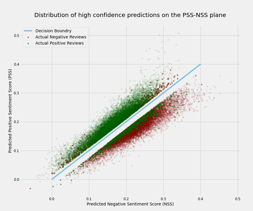
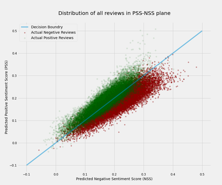
# Let's visualize the data to understand the results better. In the below scatter plot each review has been placed on the plane based on its PSS and NSS. Therefore, all points above the decision boundary (diagonal blue line) have positive S3 and are then predicted to have a positive sentiment and all points below the boundary have negative S3 and are thus predicted to have a negative sentiment. The actual sentiment labels of reviews are shown by green (positive) and red (negative). It is evident from the plot that most mislabelings happen close to the decision boundary as expected.  

# ![alt text](../reports/figures/distribution_of_all_reviews_in_PSS_NSS_plane_TopSSA.png)

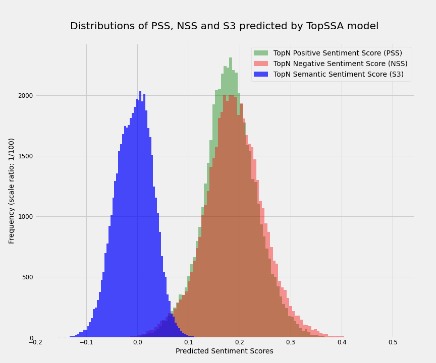
# ## High confidence predictions
# It is well-known that the results further from the decision boundary have better performance. Here I show that this applies to our unsupervised model as well. To do so, I plotted the distribution of the S3, PSS, and NSS for all reviews. As we would expect from Central Limit Theorem, all three distributions are very close to normal with S3 having a mean and std of -0.003918 and 0.037186 respectively. Next, I define the high confidence predictions to be those that their S3 is at least `0.5*std` away from the mean. That consists of ~64% of reviews and the model has the F1 of ~94% for them. 

# ![alt text](../reports/figures/pss_nss_s3_Distributions.png)

# ![alt text](../reports/figures/distribution_of_high_confidence_predictions_on_PSS_NSS_plane.png)

# ---
# [Back to top ^](#Table_of_contents)
# 
# <a id='Further_Analysis'></a> 
# # 5. Further Analysis
# ---

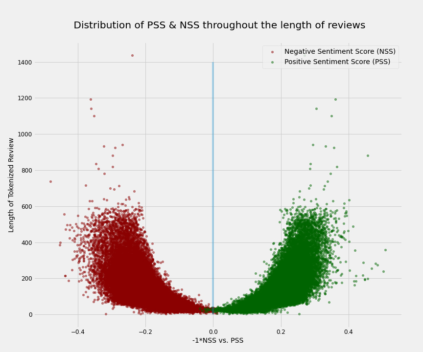
# So far, I showed how a simple unsupervised model can perform very well on a sentiment analysis task. As I promised in the introduction, now I will show how this model will be able to provide additional valuable information that supervised models are not providing. Namely, I will show that this model can give us an understanding of the sentiment complexity of the text. To do so, I will again rely on our positive and negative scores. First, let's look into another property of those scores. In addition to the fact that both scores are normally distributed, their values are correlated with the length of the review. Namely, the longer the review, the higher its negative and positive scores. A simple explanation is that with more words, one can potentially express more positive or negative emotions. Of course, the scores cannot be more than 1 and they saturate eventually (around 0.35 here). The below plot shows the correlation very well. Please note that in order to better depict this for both PSS and NSS, I reversed the sign of NSS values.

# ![alt text](../reports/figures/pss_nss_distribution_throughout_length.png)

# 
# Therefore to account for the effect of text length in our analysis, we slice the dataset so that reviews placed in each subset would be close in length. In this post, I limit the analysis to the reviews between 100 to 140 tokens (the average number of tokens in reviews is 120). This slice has around 8400 datapoints in it and their respective F1 score is ~82%, which is close to the F1 score on the whole dataset. Additionally, both PSS and NSS in this slice have a normal distribution with the following values:
# 
# > PSS_mean = 0.200648  
# > PSS_std = 0.031200
# 
# > NSS_mean = 0.205617  
# > NSS_std = 0.039358 
# 
# From now on, any mention of mean and std of PSS and NSS refers to the values in this slice of the dataset.

# In[17]:


df_slice = df[df["tokenized_text_len"].between(100,140)]
len(df_slice)


# ## Sentiment Complexity
# 
# My main claim here is that we can assess the sentiment complexity (or complexity of emotions) of a text using their PSS and NSS. I will show that if a text has simultaneously high PSS and high NSS values (low S3), it probably has a high sentiment complexity. And a text with a low PSS and a high NSS value or vice versa (high S3), could be considered as having a more clear sentiment or a low sentiment complexity. But first, we should define high and low. For the sake of this analysis we define high and low PSS (NSS) to be values above and below one standard deviation from their mean respectively, but of course these definitions are relative and could be adjusted. So
# 
# 
# >- High PSS(NSS) = PSS(NSS) > mean_PSS(NSS) + std_PSS(NSS)
# >-  Low PSS(NSS) = PSS(NSS) < mean_PSS(NSS) - std_PSS(NSS)
# 
# Therefore the high sentiment complexity could be defined as:
# 
# > High sentiment complexity = High PSS & High NSS
# 
# In contrast, there is a group of reviews that have simultaneously low PSS and low NSS. These reviews often state Less opinions and more facts, so they could be called reviews with Low subjectivity, and be quantitatively defined as
# 
# > Low Subjectivity = low PSS & low NSS
# 
# The plot below shows how these two groups of reviews are distributed on the PSS-NSS plane.

# ![alt text](../reports/figures/low_subjectivity_vs_high_complexity_reviews_on_PSS_NSS_plane.png)

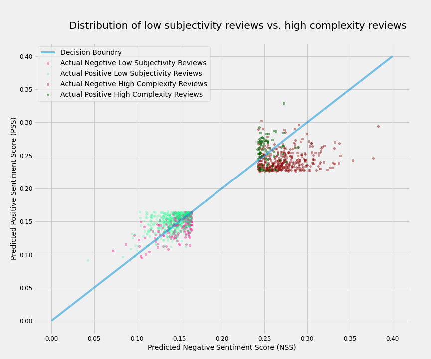
# Although for both the high sentiment complexity group and the low subjectivity group, the S3 does not necessarily fall around the decision boundary, yet -for different reasons- it is harder for our model to predict their sentiment correctly. Traditional classification models cannot differentiate between these two groups, but our approach provides us with this extra information. The following two interactive plots let you explore the reviews by hovering over them.

# In[18]:


explore_high_complexity_reviews(df_slice)


# In[19]:


explore_low_subjectivity_reviews(df_slice)


# ## A Qualitative Assessment

# In the rest of this post, I will qualitatively analyze a couple of reviews from the high complexity group  to support my claim that sentiment analysis is a complicated intellectual task even for the human brain.
# 
# Although NLP is never concerned with relation between intention and convention in a way that this issue is addressed in theory of meaning and philosophy of language, we can not ignore that one may use words with an intention of meaning or sentiment that differs from the ordinary usages of the words. For instance, we may sarcastically use a word, which is often considered positive in convention of communication to express our negative opinion. A sentiment analysis model can not notice this sentiment shift if it did not learn how to use contextual indications to predict sentiment intended by the author. To illustrate this point let's see review **#46798** which has minimum S3 in the high complexity group. Starting with the word "Wow" which is the exclamation of surprise, often used for expressing astonishment or admiration, the review seems to be a positive one. The reviewer paradoxically repeats that bad films are entertaining. But the model successfully captured the negative sentiment expressed with irony and sarcasm. 
# 
# Another reason behind the sentiment complexity of a text is to express different emotions about different aspects of the subject so that the general sentiment of the text would not be clearly grasped. An instance is review  **#21581** that has the highest S3 in the group of high sentiment complexity. The review starts with the story of the film which is, according to the reviewer, "so stupid" and "a poor joke, at best". But soon after that, the complexity appears by stating positive and negative aspects of the film using several *sentiment shifters* such as 'not', 'but' and 'however'. Overall the film is 8/10 in the reviewer's opinion and the model managed to predict this positive sentiment despite all the complex emotions expressed in this short text. In contrast,  review **#29090** is an example of the model's error. The review is strongly negative and clearly expresses disappointment and anger about the ratting and publicity that the film gained undeservedly. However, the model failed to predict the sentiment. Apparently, because the review vastly includes other people's positive opinions on the movie as well as the reviewer's positive emotions on other movies.
# 
# Similarly interesting, review **#16858** dramatically combines complex emotions about the film. The reviewer used to love the film and watched it over and over when they were a kid. Watching the film as a grown-up, their experience, however, isn't as great as they remembered: the acting, the storyline, the jokes look "pretty bad". No one can be sure about the reviewer's final decision between these two completely opposite sentiments. And surprisingly they decide to appreciate their childhood and give it 7 stars. No wonder that the model failed to recognize the power of nostalgia.
# 
# To be fair, we must admit that sometimes our manual labeling is also not accurate enough. An impressive example is review **#46894** which is labeled as negative but the reviewer explicitly spells out that "I give the show a six". Please note that the dataset introduction document claims that reviews with scores 5 and 6 are considered neutral and not included in the dataset. Nevertheless, our model accurately classified this review as positive although in model evaluation we had to count it as a false positive prediction. 

# **Review #46798 (True Negative Prediction):**
# - `topn_PSS` = 0.297876
# - `topn_NSS` = 0.389544
# - `topn_semantic_sentiment_score` = -0.0916676 
# 
# > "Wow. As soon as I saw this movie\'s cover, I immediately wanted to watch it because it looked so bad. Sometimes I watch Bollywood movies just because they\'re so bad that it will be entertaining (eg. Koi Mil Gaya). This movie had all the elements of an atrocious film: a "gang of local thugs" that is completely harmless, a poorly done motorcycle scene, horrible dialouge ("Congrats son, I am very proud that you are a Bad Boy"), actors playing basketball as if they are good, atrocious songs ("Me bad, me bad, me bad bad boy"), unexplained plot lines like why are the Good Boy and Bad Boy friends??? And why is the hot girl in love with the nerd?? I\'ve never seen such a poorly constructed story with such horrible directly. Some of the scenes actually took 30 seconds long like the one where the Good and Bad Boys inexplicably ran over the "gang member\'s" poker game. Congrats Ashwini Chaudry, you are a Bad Director. If you want to watch a good movie, watch Guru, if you want to watch a movie so bad that it\'s actually entertaining, then watch Good Boy, Boy."

# **Review #21581 (True Positive Prediction):**
# - `topn_PSS` = 0.260054
# - `topn_NSS` = 0.247708
# - `topn_semantic_sentiment_score` = 0.0123464
# 
# > "The plot: A crime lord is uniting 3 different mafias in an entreprise to buy an island, that would then serve as money-laundering facility for organized crime. To thwart that, the FBI tries to bust one of the mafia lords. The thing goes wrong, and by some unlikely plot twists and turns, we are presented with another "cop buddies who don\'t like each other" movie... one being a female FBI agent, and the other a male ex-DEA agent.<br /><br />So far, so stupid. But the strength of this movie does not lie in its story - a poor joke, at best. It is funny. (At least the synchronized German version is). The action is good, too, with a memorable scene involving a shot gun and a rocket launcher. But the focus is squarely on the humour. Not intelligent satire, not quite slapstick, but somewhere in between, you get a lot of funny jokes. <br /><br />However, this film is the opposite of political correctness. Legal drug abuse is featured prominently, without criticism, and even displaying it as cool. That\'s the bit of the movie that seriously annoyed me, and renders it unsuitable for kids, in my opinion. <br /><br />All in all, for a nice evening watching come acceptable action with some funny jokes, this movie is perfect. Just remember: In this genre, it is common to leave your brain at the door when you enter the cinema / TV room. Then you\'ll have a good time. 8/10"

# **Review #29090 (False Positive Prediction):**
# 
# - `topn_PSS` = 0.254718
# - `topn_NSS` = 0.252167
# - `topn_semantic_sentiment_score` = 0.00255111
# 
# > "How this film gains a 6.7 rating is beyond belief. It deserves nothing better than a 2.0 and clearly should rank among IMDb\'s worst 100 films of all time. National Treasure is an affront to the national intelligence and just yet another assault made on American audiences by Hollywood. Critics told of plot holes you could drive a 16 wheeler through.<br /><br />I love the justifications for this movie being good... "Nicholas Cage is cute." Come on people, no wonder people around the world think Americans are stupid. This has to be the most stupid, insulting movie I have ever seen. If you wanted to see an actually decent film this season, consider Kinsey, The Woodsman, Million Dollar Baby or Sideways. National Treasure unfortunately got a lot more publicity than those terrific films. I bet most of you reading this haven\'t even heard of them, since some haven\'t been widely released yet.<br /><br />Nicholas Cage is a terrific actor - when he is in the right movies. Time after time I\'ve seen Cage waste his terrific talent in awful mind-numbing films like Con Air, The Rock and Face-Off. When his talent is put to good use like in Charlie Kaufman\'s Adaptation he is an incredible actor.<br /><br />Bottom line - I\'d rather feed my hand to a wood chipper than be subjected to this visual atrocity again."

# **Review #16858 (False Negative Prediction):**
# - `topn_PSS` = 0.251645
# - `topn_NSS` = 0.256545
# - `topn_semantic_sentiment_score` = -0.0048998
# 
# >"Yes, I loved this movie when I was a kid. When I was growing up I saw this movie so many times that my dad had to buy another VHS copy because the old copy had worn out.<br /><br />My family received a VHS copy of this movie when we purchased a new VHS system. At first, my mom wasn't sure that this was an appropriate movie for a 10 year old but because we had just bought a new VHS system she let me watch it.<br /><br />Like I said, this movie is every little boys dream The movie contains a terrific setting, big muscled barbarians, beautiful topless women, big bad monsters and jokes you'll only get when you get older. So, a couple of days ago I inserted the video and watched the movie again after a long time. At first, I was bored, then started thinking about how much I loved this movie when I was kid, and continued watching. Yeah, the experience wasn't as great as I remembered The acting is pretty bad, the storyline is pretty bad, the jokes weren't funny anymore, but the women were still pretty. Yes, I've grown up. Even though the movie experience has changed for me, I still think it's worth 7 stars. For the good old times you know"

# **Review #46894 (Positive Prediction, wrongly labeled as Negative)**:
# - `topn_PSS` = 0.286535
# - `topn_NSS` = 0.211566
# - `topn_semantic_sentiment_score` = 0.0749689
# >"I give the show a six because of the fact that the show was in fact a platform for Damon Wayans as the Cosby Show was for Bill Cosby, it dealt with a lot of issues with humor and I felt that it in fact tailored to getting a laugh as opposed to letting the jokes come from the character. <br /><br />Michael Kyle An interesting patriarch and a wisecracking person. He is PHENOMENAL in movies, but in the show he was there for the wisecrack and though I loved it, I felt that the laugh was more important than plausibility.<br /><br />Jay Kyle I have loved her since House Party and have enjoyed her in School Daze and Martin, this was a great role for her and she made a great choice in picking this sitcom to co-star in. I also feel that Jay and Michael were more like equals in the show but Jay was more the woman who fed her crazy husbands the lines and went along with his way of unorthodox discipline because she may have felt that it worked<br /><br />Jr Just plain stupid, his character should have been well developed and even though he does have his moments of greatness, we are returned to the stupidity as if he learned nothing, which drives me nuts!!!!!!!! Not to mention that most of the situations (in episodes I've seen) seems to center around him<br /><br />Clair The attractive sister who dated a Christian, I found her boyfriend's character to be more interesting than she was (she'd be better off sticking to movies, the writers should have done more to show her intelligence but it's not stereotypical enough)<br /><br />Kady Lovable and the youngest daughter. I think the writers established her character most on the show aside from the parents and Franklin<br /><br />Franklin I LOVE this character and I think they derived it from Smart Guy (T.J. Mowry) which only lasted one season. They did a great job of casting for this little genius (the effort would have been made if Jr would have been the smart one but show the down sides also)<br /><br />All in all, this sitcom is a wonderful thing and it's homage to the Cosby Show is well done, I love the show and wished it would have stayed on longer than that. I can't wait to see the series finale"

# ### Now it's your turn
# Let's have fun with the *Text Semantic Sentiment Analysis* function. Share your opinion with the TopSSA model and explore how accurate is it in analyzing the sentiment.

# In[ ]:


text_SSA(keyed_vectors=keyed_vectors,
              tokenizer=tokenizer,
              positive_target_tokens=pos_concepts,
              negative_target_tokens=neg_concepts,
              topn=30)


# ---
# ## Acknowledgments
# I’d like to express my deepest gratitude to [Javad Hashemi](https://www.linkedin.com/in/thejavadhashemi/) for his constructive suggestions and helpful feedback on this project. Particularly, I am grateful for his insights on sentiment complexity and his optimized solution to calculate vector similarity between two lists of tokens that I used in the [`list_similarity`](https://github.com/TextualData/IMDB-Semantic-Sentiment-Analysis/blob/main/Word2Vec/src/w2v_utils.py) function.