#!/usr/bin/env python
# coding: utf-8
# # Tensor Parallelism
# 이번 세션에서는 Tensor parallelism에 대해서 알아보겠습니다.
# ## 1. Intra-layer model parallelism
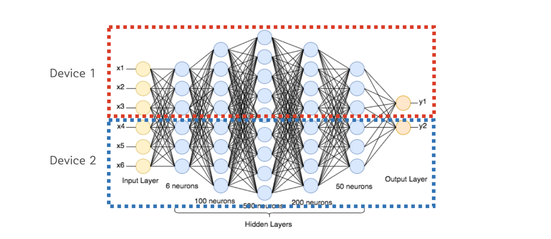
# Tensor Parallelism은 Intra-layer 모델 병렬화 방식으로 **레이어 내부에서 텐서 단위로 모델을 쪼갭니다.** Inter-layer 모델 병렬화는 상식적으로 이해가 가지만, Intra-layer 병렬화의 경우는 처음 보시는 분들은 어떻게 이 것이 가능한지 궁금하실거에요.
#
# 
#
# 우리가 흔히 사용하는 내적 연산은 연산하고자 하는 행렬을 쪼개서 병렬적으로 수행하고 결과를 더하거나 이어붙여도 최종 출력값이 변하지 않는 성질이 있습니다. 이러한 내적 연산의 성질을 이용하여 모델을 병렬화 하는것을 Tensor 병렬화라고 합니다. 용어가 다소 헷갈릴 수 있는데 Intra-layer는 레이어 단위에서 일어나지 않는 모든 병렬화를 의미하기 때문에 더 큰 범주이고, Tensor 병렬화는 Intra-layer 병렬화의 구현하는 방법 중 한가지 입니다.
# ## 2. Megatron-LM
# Megatron-LM은 NVIDA에서 공개한 Intra-layer 모델 병렬화 구현체로, 현재 Large-scale 모델 개발에 있어서 가장 중요한 프로젝트 중 하나입니다.
#
#  #
# ### Column & Row parallelism
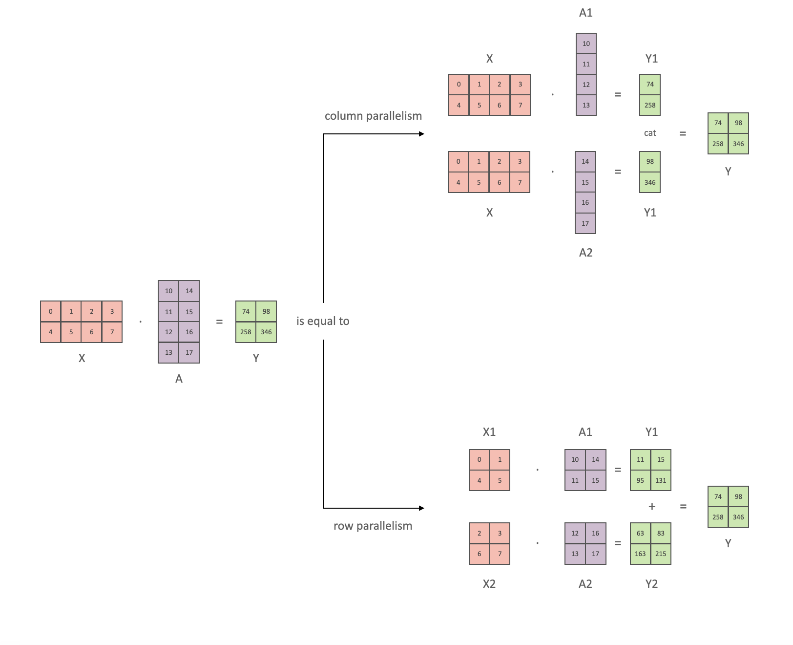
# 다음은 Megatron-LM에서 사용되는 column parallelism과 row parallelism을 그림으로 나타낸 것입니다.
#
# - Column parallelism은 **모델의 파라미터(A)를 수직방향으로 분할(A1, A2)하는 방법**입니다.
# - Row parallelism은 **모델의 파라미터(A)를 수평방향으로 분할(A1, A2)하는 방법**입니다.
#
# 
#
# 직접 코딩해서 결과를 확인해봅시다. 가장 먼저 텐서 X와 텐서 A의 행렬곱 결과는 다음과 같습니다.
# In[1]:
"""
src/non_parallelism.py
"""
import torch
X = torch.tensor(
[
[0, 1, 2, 3],
[4, 5, 6, 7],
]
)
A = torch.tensor(
[
[10, 14],
[11, 15],
[12, 16],
[13, 17],
]
)
Y = X @ A
print(Y)
# column parallelism은 모델의 파라미터(A)를 수직방향으로 자른 뒤 연산후 연산 결과를 concat하는 방식입니다. 그림에서와 같이 X는 복제하고 텐서 A를 수직방향으로 분할한 뒤 연산 후 concat 해보겠습니다.
# In[2]:
"""
src/column_parallelism.py
"""
import torch
X = torch.tensor(
[
[0, 1, 2, 3],
[4, 5, 6, 7],
]
)
A1 = torch.tensor(
[
[10],
[11],
[12],
[13],
]
)
A2 = torch.tensor(
[
[14],
[15],
[16],
[17],
]
)
Y1 = X @ A1
Y2 = X @ A2
print(Y1)
print(Y2)
Y = torch.cat([Y1, Y2], dim=1)
print(Y)
# 병렬화 전 후의 연산 결과가 동일한 것을 확인 할 수 있습니다.
#
# 그 다음으로 row parallelism를 알아봅시다. row parallelism은 모델의 파라미터(A)를 수평방향으로 분할 한 뒤 연산 결과를 더하는 방식입니다. 그림과 같이 X와 Y 모두를 분할한 뒤 연산 후 결과 값을 더해보겠습니다.
# In[3]:
"""
src/row_parallelism.py
"""
import torch
X1 = torch.tensor(
[
[0, 1],
[4, 5],
]
)
X2 = torch.tensor(
[
[2, 3],
[6, 7],
]
)
A1 = torch.tensor(
[
[10, 14],
[11, 15],
]
)
A2 = torch.tensor(
[
[12, 16],
[13, 17],
]
)
Y1 = X1 @ A1
Y2 = X2 @ A2
print(Y1)
print(Y2)
Y = Y1 + Y2
print(Y)
# 연산 결과가 동일한 것을 확인할 수 있습니다.
#
#
#
# ### Column & Row parallelism
# 다음은 Megatron-LM에서 사용되는 column parallelism과 row parallelism을 그림으로 나타낸 것입니다.
#
# - Column parallelism은 **모델의 파라미터(A)를 수직방향으로 분할(A1, A2)하는 방법**입니다.
# - Row parallelism은 **모델의 파라미터(A)를 수평방향으로 분할(A1, A2)하는 방법**입니다.
#
# 
#
# 직접 코딩해서 결과를 확인해봅시다. 가장 먼저 텐서 X와 텐서 A의 행렬곱 결과는 다음과 같습니다.
# In[1]:
"""
src/non_parallelism.py
"""
import torch
X = torch.tensor(
[
[0, 1, 2, 3],
[4, 5, 6, 7],
]
)
A = torch.tensor(
[
[10, 14],
[11, 15],
[12, 16],
[13, 17],
]
)
Y = X @ A
print(Y)
# column parallelism은 모델의 파라미터(A)를 수직방향으로 자른 뒤 연산후 연산 결과를 concat하는 방식입니다. 그림에서와 같이 X는 복제하고 텐서 A를 수직방향으로 분할한 뒤 연산 후 concat 해보겠습니다.
# In[2]:
"""
src/column_parallelism.py
"""
import torch
X = torch.tensor(
[
[0, 1, 2, 3],
[4, 5, 6, 7],
]
)
A1 = torch.tensor(
[
[10],
[11],
[12],
[13],
]
)
A2 = torch.tensor(
[
[14],
[15],
[16],
[17],
]
)
Y1 = X @ A1
Y2 = X @ A2
print(Y1)
print(Y2)
Y = torch.cat([Y1, Y2], dim=1)
print(Y)
# 병렬화 전 후의 연산 결과가 동일한 것을 확인 할 수 있습니다.
#
# 그 다음으로 row parallelism를 알아봅시다. row parallelism은 모델의 파라미터(A)를 수평방향으로 분할 한 뒤 연산 결과를 더하는 방식입니다. 그림과 같이 X와 Y 모두를 분할한 뒤 연산 후 결과 값을 더해보겠습니다.
# In[3]:
"""
src/row_parallelism.py
"""
import torch
X1 = torch.tensor(
[
[0, 1],
[4, 5],
]
)
X2 = torch.tensor(
[
[2, 3],
[6, 7],
]
)
A1 = torch.tensor(
[
[10, 14],
[11, 15],
]
)
A2 = torch.tensor(
[
[12, 16],
[13, 17],
]
)
Y1 = X1 @ A1
Y2 = X2 @ A2
print(Y1)
print(Y2)
Y = Y1 + Y2
print(Y)
# 연산 결과가 동일한 것을 확인할 수 있습니다.
#
#
#
# ### Column parallelism: $(D, D) → (D, \frac{D}{n}) \times n$
#
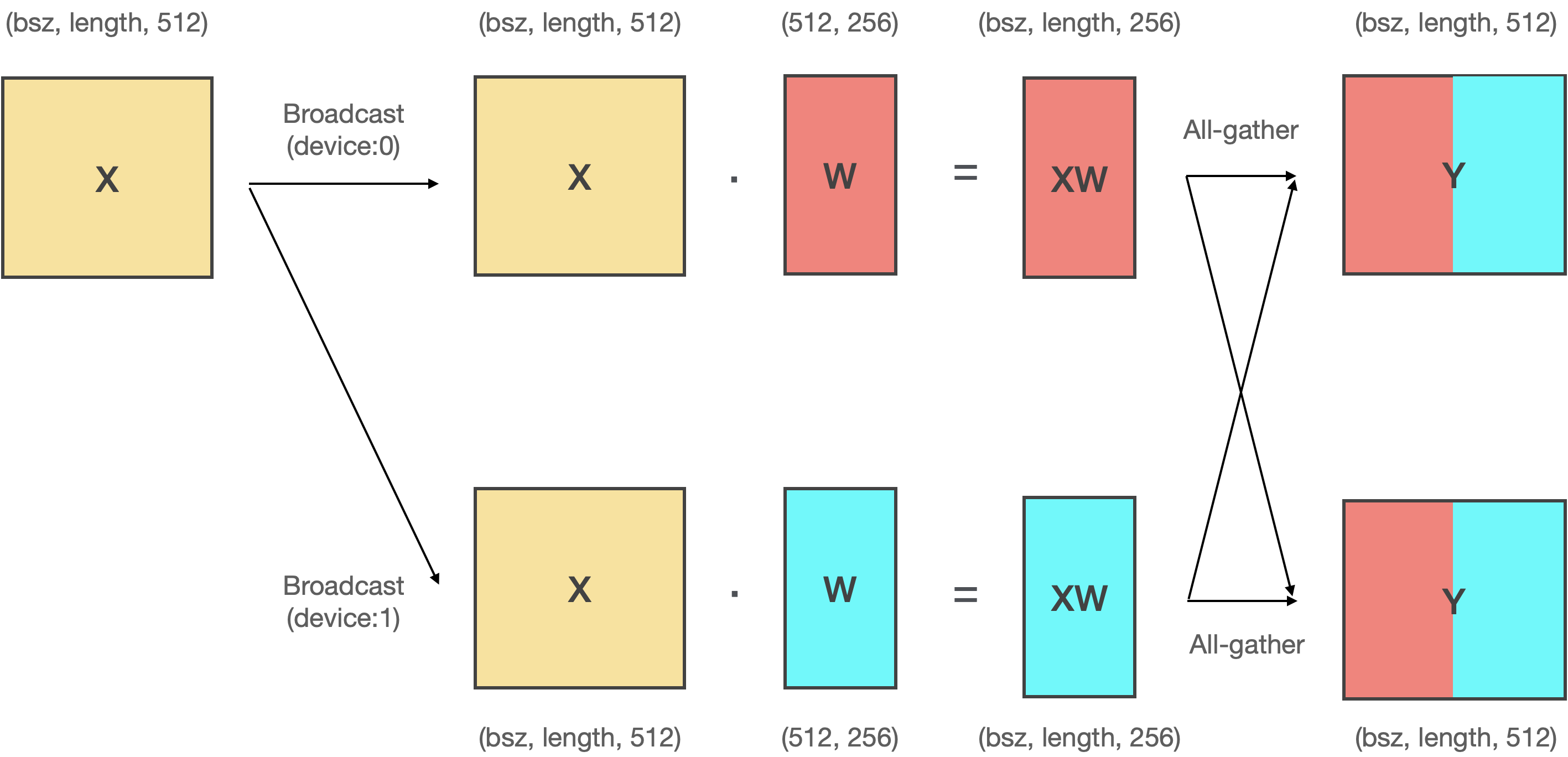
# 앞선 예시에서 본 것 처럼, Column Parallelism은 **입력텐서(X)를 복사**하고, 모델의 파라미터(A)를 **수직방향으로 분할(A1, A2)하여 내적** 후 concat하는 연산입니다.
#
#
#
# 
#
#
#
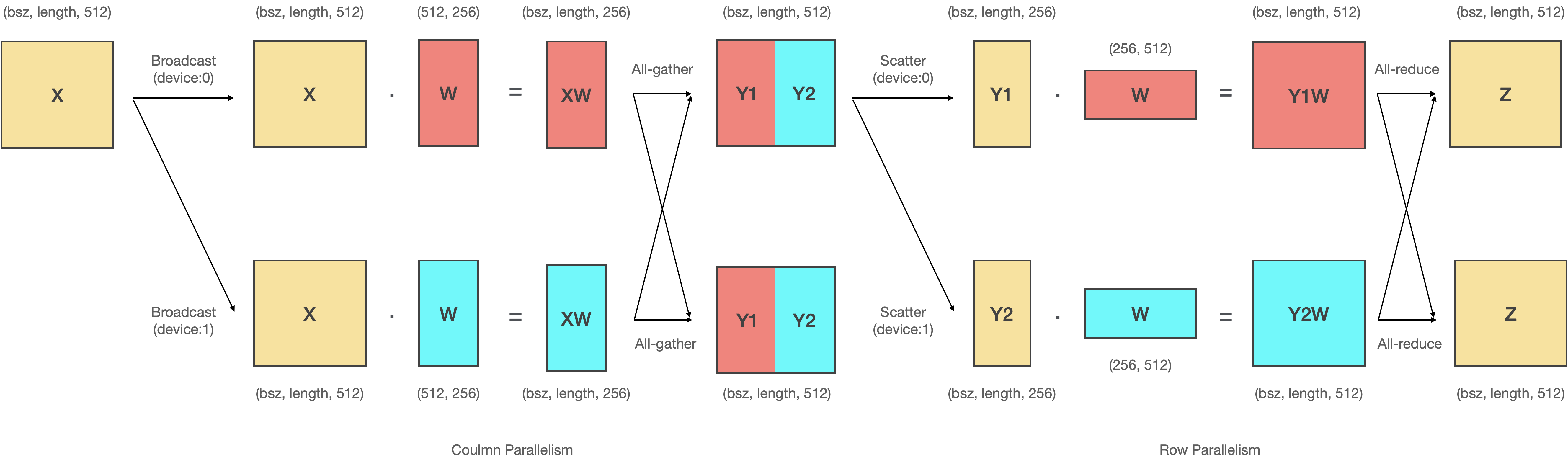
# Megatron-LM에서는 **분할된 파라미터 (A1, A2)를 서로 다른 디바이스에 올려서 모델을 병렬화** 합니다. 이에 따라 행렬 곱 연산도 여러개의 GPU에서 동시에 일어나게 되고, 이를 처리하기 위해 분산 프로그래밍이 필요합니다. Column Parallelism을 위해서는 Broadcast와 All-gather 연산을 사용합니다.
#
# - 서로 다른 GPU에 동일한 입력을 전송하기 위해 **Broadcast** 연산를 사용합니다.
# - 행렬 곱 연산 결과를 모으기 위해 **All-gather** 연산을 사용합니다.
#
# In[ ]:
"""
참고: ColumnParallelLinear in megatron-lm/megatron/mpu/layers.py
"""
def forward(self, input_):
bias = self.bias if not self.skip_bias_add else None
# Set up backprop all-reduce.
input_parallel = copy_to_tensor_model_parallel_region(input_)
# Matrix multiply.
output_parallel = F.linear(input_parallel, self.weight, bias)
if self.gather_output:
output = gather_from_tensor_model_parallel_region(output_parallel)
else:
output = output_parallel
output_bias = self.bias if self.skip_bias_add else None
return output, output_bias
# ### Row parallelism: $(D, D) → (\frac{D}{n}, D) \times n$
#
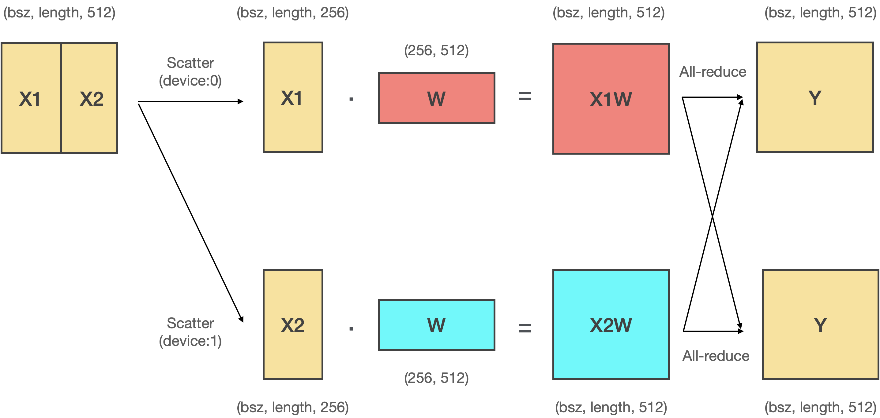
# Row Parallelism은 **입력텐서(X)를 분할**하고, 모델의 파라미터(A)를 **수평방향으로 분할(A1, A2)하여 내적** 후 더하는 연산입니다.
#
#
#
# 
#
#
#
# 마찬가지로 Row Parallelism을 여러 GPU에서 실행하기 위해서는 분산 프로그래밍이 필요합니다. Row Parallelism을 위해서는 Scatter와 All-reduce을 사용합니다.
#
# - 서로 다른 GPU에 입력을 분할하여 전송하기 위해 **Scatter** 연산를 사용합니다.
# - 행렬 곱 연산 결과를 더하기 위해서 **All-reduce** 연산을 사용합니다.
#
# In[ ]:
"""
참고: RowParallelLinear in megatron-lm/megatron/mpu/layers.py
"""
def forward(self, input_):
# Set up backprop all-reduce.
if self.input_is_parallel:
input_parallel = input_
else:
input_parallel = scatter_to_tensor_model_parallel_region(input_)
# Matrix multiply.
output_parallel = F.linear(input_parallel, self.weight)
# All-reduce across all the partitions.
output_ = reduce_from_tensor_model_parallel_region(output_parallel)
if not self.skip_bias_add:
output = output_ + self.bias if self.bias is not None else output_
output_bias = None
else:
output = output_
output_bias = self.bias
return output, output_bias
#
# ### Transformer Block
#
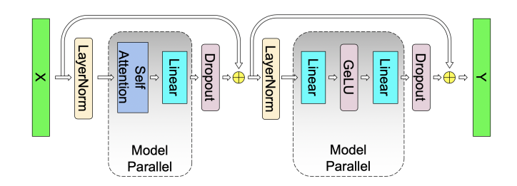
# 이제 Column, Row parallelism에 대해 이해했으니 본격적으로 어떻게 Transformer를 병렬화 할지 살펴봅시다. 우리가 흔히 아는 Transformer Block은 다음과 같이 구성되어 있습니다. Megatron-LM은 여기에서 파라미터의 크기가 매우 적은 Layer Norm 레이어는 파라미터를 모든 디바이스로 복제하고, Layer Norm 레이어를 제외한 다른 레이어들(Attention, MLP)은 위와 같이 Column, Row parallelism을 통해 병렬처리를 수행합니다.
#
# 
#
#
#
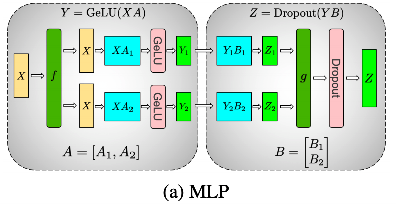
# ### MLP Layer
#
# 가장 먼저 MLP 레이어에 대해 알아보겠습니다. MLP 레이어는 `Linear1` → `GeLU` → `Linear2` → `Dropout`순으로 진행됩니다.
#
#
#
# 
#
#
#
#
# In[ ]:
"""
참고 transformers/models/gpt_neo/modeling_gpt_neo.py
"""
import torch.nn as nn
class GPTNeoMLP(nn.Module):
def __init__(self, intermediate_size, config): # in MLP: intermediate_size= 4 * hidden_size
super().__init__()
embed_dim = config.hidden_size
self.c_fc = nn.Linear(embed_dim, intermediate_size)
self.c_proj = nn.Linear(intermediate_size, embed_dim)
self.act = ACT2FN[config.activation_function]
self.dropout = nn.Dropout(config.resid_dropout)
def forward(self, hidden_states):
hidden_states = self.c_fc(hidden_states)
hidden_states = self.act(hidden_states)
hidden_states = self.c_proj(hidden_states)
hidden_states = self.dropout(hidden_states)
return hidden_states
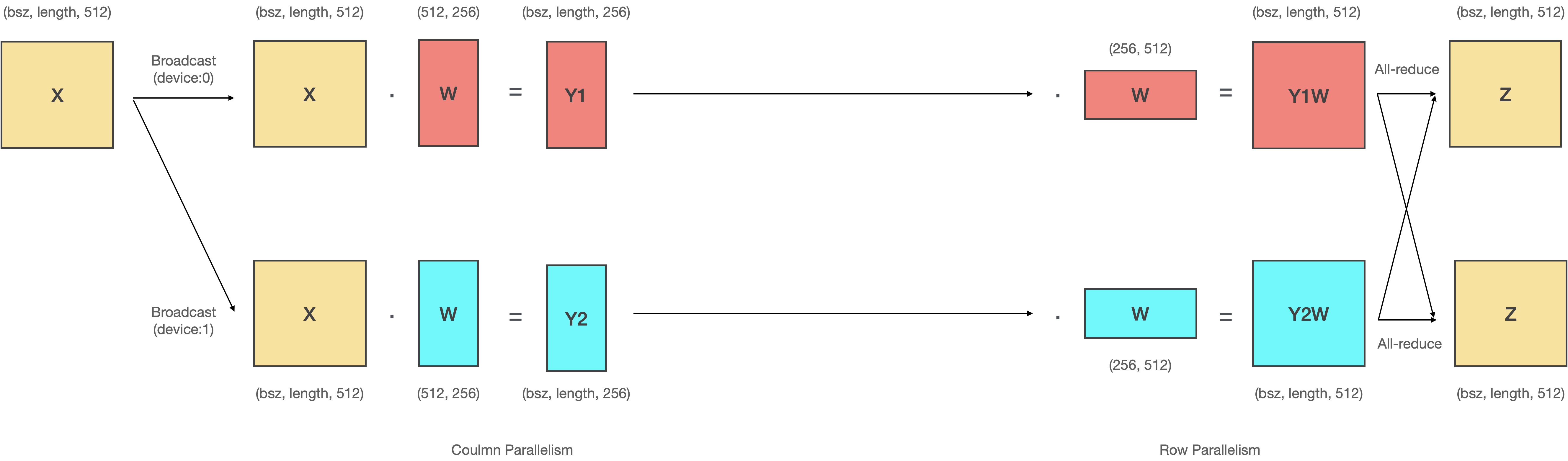
# 여기에서 **첫번째 Linear는 Coulmn Parallelism**을, **두번째 Linear는 Row Parallelism**을 적용합니다.
#
#
#
# 
#
#
#
# MLP 레이어에서 Column-Row 순으로 병렬화를 적용하는 이유는 두가지가 있습니다.
#
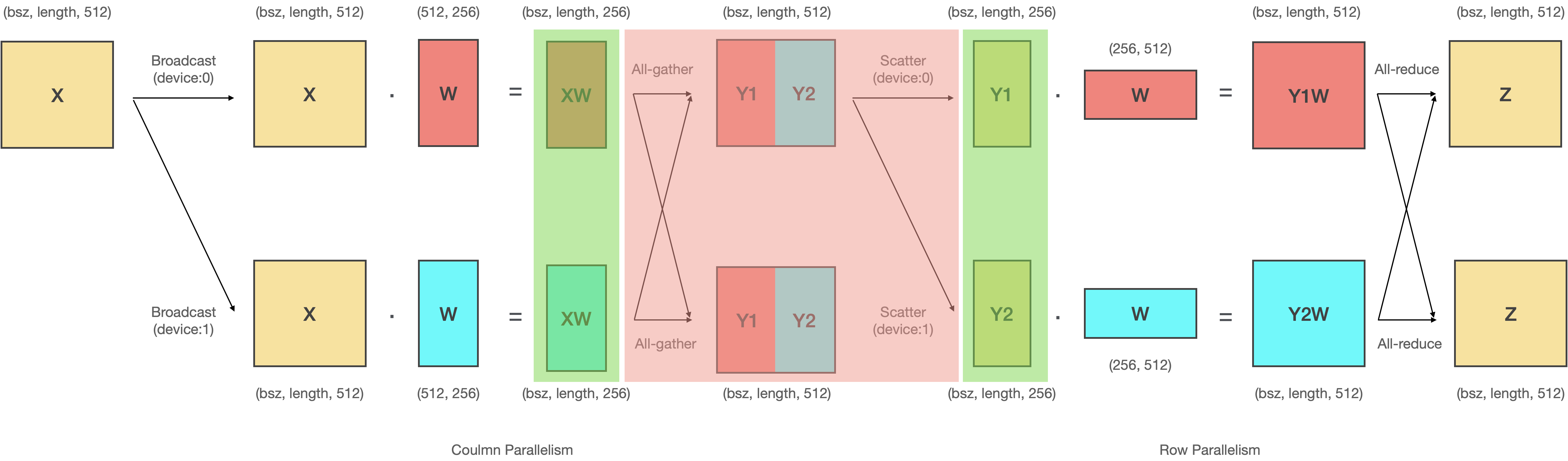
# - 첫번째 이유는 **`All-gather` 연산과 `Scatter` 연산을 생략** 할 수 있기 때문입니다.
#
#
#
# 
#
#
#
# 왼쪽 녹색 영역의 연산 결과는 입 력데이터 X와 각 디바이스로 병렬화된 W를 내적한 것입니다. 그리고 나서 붉은색 영역에서 이 결과값을 `All-gather`해서 이어붙인 다음에 다시 `Scatter`하여 쪼개죠. 여기에서 흥미로운 사실은 이어 붙인 텐서를 다시 쪼갰기 때문에 이는 이어붙이기 전과 동일하다는 것입니다. 따라서 오른쪽의 녹색 영역과 왼쪽의 녹색영역 값은 동일하죠. 결과적으로 붉은색 영역 (`All-gather`-`Scatter`)을 생략할 수 있고, 속도 면에서 큰 이득을 가져올 수 있습니다.
#
# 이는 Column-Row 순으로 병렬화 할때만 나타나는 독특한 현상으로, 만약 Column-Column, Row-Column, Row-Row와 같이 병렬화 한다면 두 Linear 레이어 사이에서 발생하는 통신을 생략할 수 없게 됩니다.
#
#
#
# 
#
#
#
# `All-gather`와 `Scatter`를 생략하는 기법은 Megatron-LM에 `input_is_parallel`와 `gather_output`라는 파라미터로 구현되어있습니다.
# In[ ]:
"""
참고: ColumnParallelLinear in megatron-lm/megatron/mpu/layers.py
"""
def forward(self, input_):
bias = self.bias if not self.skip_bias_add else None
# Set up backprop all-reduce.
input_parallel = copy_to_tensor_model_parallel_region(input_)
# Matrix multiply.
output_parallel = F.linear(input_parallel, self.weight, bias)
# gather_output을 False로 설정하여 output을 병렬화된 채로 출력합니다.
if self.gather_output:
output = gather_from_tensor_model_parallel_region(output_parallel)
else:
output = output_parallel
output_bias = self.bias if self.skip_bias_add else None
return output, output_bias
"""
참고: RowParallelLinear in megatron-lm/megatron/mpu/layers.py
"""
def forward(self, input_):
# Set up backprop all-reduce.
# input_is_parallel True로 설정하여 input을 병렬화된 채로 입력받습니다.
if self.input_is_parallel:
input_parallel = input_
else:
input_parallel = scatter_to_tensor_model_parallel_region(input_)
# Matrix multiply.
output_parallel = F.linear(input_parallel, self.weight)
# All-reduce across all the partitions.
output_ = reduce_from_tensor_model_parallel_region(output_parallel)
if not self.skip_bias_add:
output = output_ + self.bias if self.bias is not None else output_
output_bias = None
else:
output = output_
output_bias = self.bias
return output, output_bias
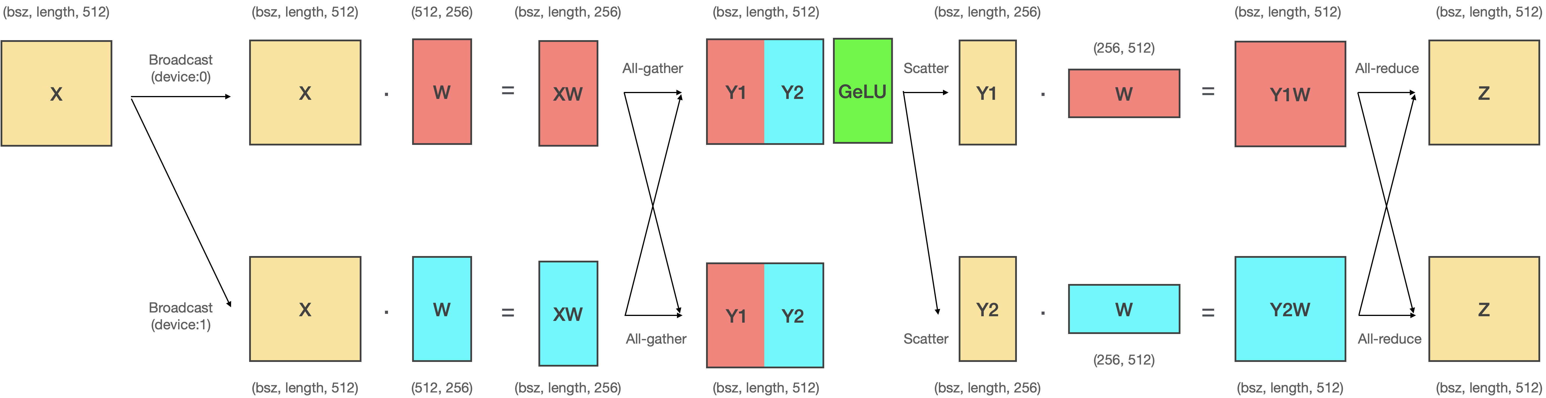
# - Column-Row 방식으로 병렬화하는 2번째 이유는 `Scatter`와 `All-gather`를 생략하려면 **GeLU 연산**이 병렬화된 채로 수행되어야 하기 때문입니다.
#
#
#
# 
#
#
#
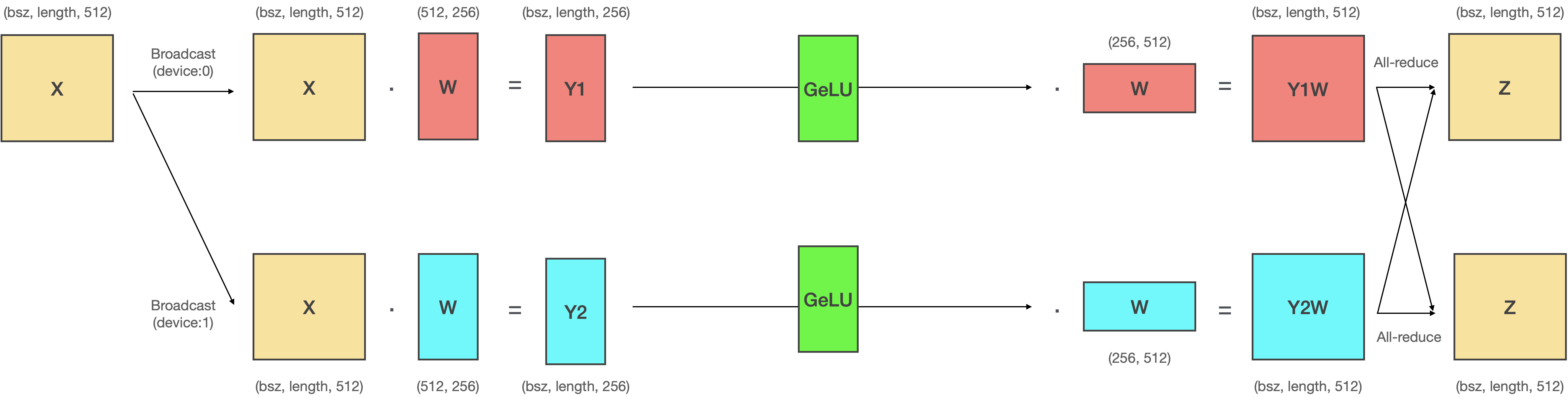
# 위 그림은 `Scatter`와 `All-gather`를 생략하지 않는 상황에서 GeLU 연산을 두 Linear 레이어 사이에 삽입한 것입니다. 만약 여기에서 두 연산을 생략하도록 구현하면 아래와 같이 GeLU 연산은 반드시 각각의 디바이스에서 이루어져야 합니다.
#
#
#
# 
#
#
#
# 그러나 이렇게 GeLU 연산을 서로 다른 디바이스에서 하도록 병렬화 시키려면 반드시 병렬적으로 계산된 GeLU의 출력은 병렬화 되지 않은 상태에서 계산된 GeLU의 출력과 동일해야겠죠. 즉 다음과 같은 공식이 성립해야 합니다. ($\circledcirc$ 기호는 concatenation을 의미합니다.)
#
#
#
# $$Row Paralleism: GeLU(XW1 + XW2) = GeLU(XW1) + GeLU(XW2)$$
#
#
#
# $$Column Paralleism: GeLU(XW1 \circledcirc XW2) = GeLU(XW1) \circledcirc GeLU(XW2)$$
#
#
#
# 문제는 위와 같은 공식이 Column Parallelism에서만 성립하고, **Row Parallelism 에서는 성립하지 않는다는 것**입니다.
#
#
#
# $$Row Paralleism: GeLU(XW1 + XW2) \neq GeLU(XW1) + GeLU(XW2)$$
#
#
#
# 이를 코드로 구현해서 확인해봅시다.
# In[4]:
"""
src/megatron_mlp_gelu.py
"""
import torch
from torch.nn.functional import gelu
w = torch.randn(6, 6)
x = torch.randn(6, 6)
class RowParallelLinear(torch.nn.Module):
def __init__(self):
super(RowParallelLinear, self).__init__()
chunked = torch.chunk(w, 2, dim=0)
# row parallelized parameters
self.w1 = chunked[0] # [3, 6]
self.w2 = chunked[1] # [3, 6]
def forward(self, x):
# GeLU(X1A1 + X2A2) != GeLU(X1A1) + GeLU(X2A2)
x1, x2 = torch.chunk(x, 2, dim=1)
# parallel output
y1 = gelu(x1 @ self.w1) + gelu(x2 @ self.w2)
# non-parallel output
y2 = gelu(x1 @ self.w1 + x2 @ self.w2)
return torch.all(y1 == y2)
class ColumnParallelLinear(torch.nn.Module):
def __init__(self):
super(ColumnParallelLinear, self).__init__()
chunked = torch.chunk(w, 2, dim=1)
# column parallelized parameters
self.w1 = chunked[0] # [6, 3]
self.w2 = chunked[1] # [6, 3]
def forward(self, x):
# GeLU(X1A1 cat X2A2) == GeLU(X1A1) cat GeLU(X2A2)
# parallel output
y1 = torch.cat([gelu(x @ self.w1), gelu(x @ self.w2)], dim=1)
# non-parallel output
y2 = gelu(torch.cat([(x @ self.w1), (x @ self.w2)], dim=1))
return torch.all(y1 == y2)
# Row Parallelism
print("Is GeLU in RowParallelLinear same with non-parallel = ", end="")
print(RowParallelLinear()(x).item())
# Column Parallelism
print("Is GeLU in ColumnParallelLinear same with non-parallel = ", end="")
print(ColumnParallelLinear()(x).item())
# 따라서 GeLU 연산을 병렬화 시키려면 반드시 GeLU 이전의 Linear 레이어는 Column 방향으로 병렬화 되어있어야 합니다. 따라서 Column-Row 순서로 병렬화 하는 것이 가장 효율적인 방식이죠.
#
#
# ### Multi-head Attention Layer
#
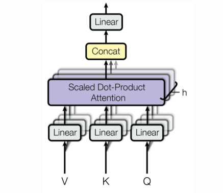
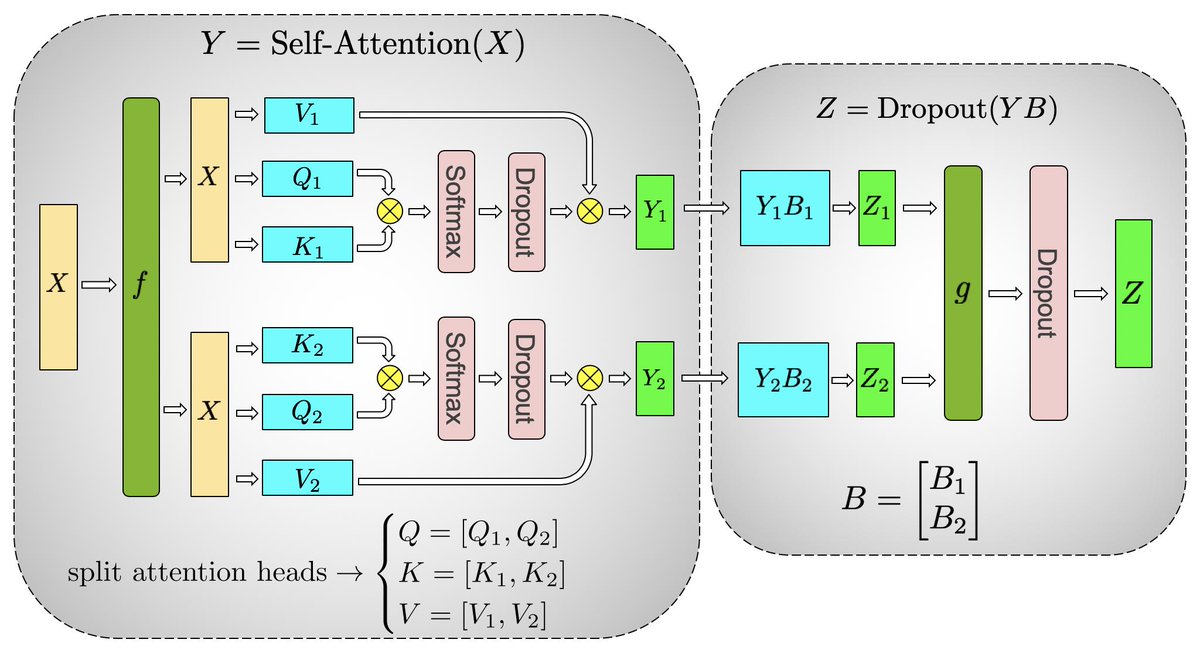
# 다음으로 Multi-head Attention 레이어에 대해 알아보겠습니다. Multi-head Attention 레이어는 `Linear1` → `Split heads` → `ScaleDotProductAttention` → `Concat(Merge) heads` → `Linear2` → `Dropout` 순으로 진행됩니다.
#
# 
#
#
# In[ ]:
"""
참고 transformers/models/gpt_neo/modeling_gpt_neo.py
"""
class GPTNeoSelfAttention(nn.Module):
def __init__(self, config, attention_type):
super().__init__()
self.attn_dropout = nn.Dropout(config.attention_dropout)
self.resid_dropout = nn.Dropout(config.resid_dropout)
self.embed_dim = config.hidden_size
self.num_heads = config.num_heads
self.head_dim = self.embed_dim // self.num_heads
if self.head_dim * self.num_heads != self.embed_dim:
raise ValueError(
f"embed_dim must be divisible by num_heads (got `embed_dim`: {self.embed_dim} and `num_heads`: {self.num_heads})."
)
self.k_proj = nn.Linear(self.embed_dim, self.embed_dim, bias=False)
self.v_proj = nn.Linear(self.embed_dim, self.embed_dim, bias=False)
self.q_proj = nn.Linear(self.embed_dim, self.embed_dim, bias=False)
self.out_proj = nn.Linear(self.embed_dim, self.embed_dim, bias=True)
def forward(
self,
hidden_states,
attention_mask=None,
layer_past=None,
head_mask=None,
use_cache=False,
output_attentions=False,
):
# 1. linear projection
query = self.q_proj(hidden_states)
key = self.k_proj(hidden_states)
value = self.v_proj(hidden_states)
# 2. split heads
query = self._split_heads(query, self.num_heads, self.head_dim)
key = self._split_heads(key, self.num_heads, self.head_dim)
value = self._split_heads(value, self.num_heads, self.head_dim)
# 3. scale dot product attention
attn_output, attn_weights = self._attn(query, key, value, attention_mask, head_mask)
# 4. concat (merge) heads
attn_output = self._merge_heads(attn_output, self.num_heads, self.head_dim)
# 5. linear projection
attn_output = self.out_proj(attn_output)
# 6. dropout
attn_output = self.resid_dropout(attn_output)
return outputs
# 
#
#
#
# Megatron-LM은 Attention 레이어의 Q, K, V Linear projection과 Output projection 부분을 병렬화 합니다. 마찬가지로 Q, K, V Linear projection 부분은 Column parallelism, Output projection 부분은 Row parallelism으로 처리하여 **Column-Row의 패턴을 만듭니다.** 이를 통해 Attention 레이어에서도 MLP 레이어와 마찬가지로 `Scatter`, `All-gather` 연산을 생략 할 수 있습니다.
#
#
# ### Vocab Parallel Embedding
#
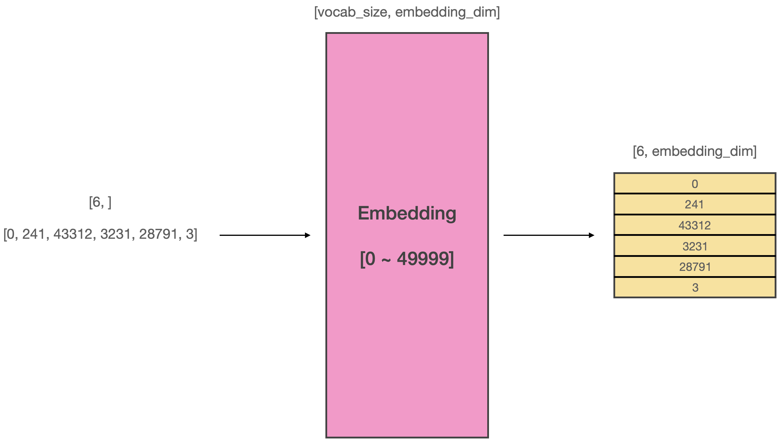
# Megatron LM은 Word embedding 레이어도 역시 병렬화 합니다. 독특한 점은 Vocab size dimension을 기준으로 병렬화 한다는 점입니다. 예를 들어 Vocab size가 50000인 Word embedding matrix가 있다고 가정하면 이 matrix의 사이즈는 (50000, embedding_dim)인 됩니다. Megatron-LM은 여기에서 Vocab size dimension을 기준으로 matrix를 병렬화 합니다. 이러한 독특한 병렬화 기법을 **Vocab Parallel Embedding**이라고 합니다.
#
# 
#
#
#
# 위 그림은 병렬화를 하지 않은 상태에서의 Word embedding을 나타냅니다. 길이가 6인 시퀀스가 입력되면 [6, embedding_dim]의 사이즈를 갖는 입력 텐서를 만듭니다.
#
#
#
# 
#
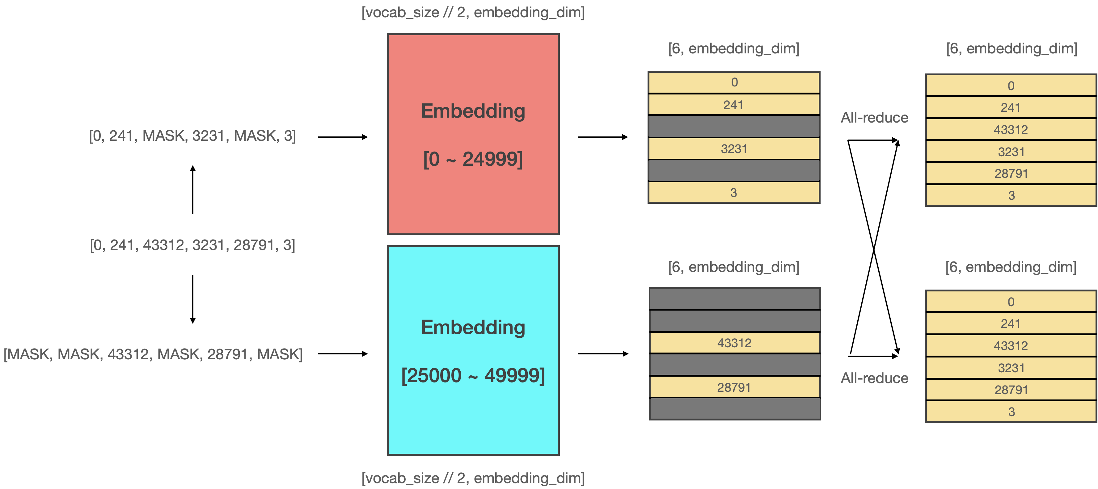
# 위 그림은 Vocab parallel embedding의 작동 방식을 나타냅니다. 기존의 임베딩 매트릭스를 절반으로 쪼개서 0번부터 24999번 토큰까지 담당하는 임베딩 매트릭스와 25000번부터 50000번 토큰까지 담당하는 임베딩 매트릭스로 분할합니다. 그리고 데이터가 들어오면 **해당 매트릭스가 커버하는 범위를 넘어서는 토큰은 마스킹**하여 처리합니다. 이후에 **마스킹 처리된 부분의 벡터는 전부 0으로 초기화** 한 뒤, 두 매트릭스를 **더하면 모든 단어의 벡터를 갖고 있는 완벽한 입력 텐서**가 됩니다.
#
# In[ ]:
"""
참고: VocabParallelEmbedding in megatron-lm/megatron/mpu/layers.py
"""
def forward(self, input_):
if self.tensor_model_parallel_size > 1:
# Build the mask.
input_mask = (input_ < self.vocab_start_index) | \
(input_ >= self.vocab_end_index)
# Mask the input.
masked_input = input_.clone() - self.vocab_start_index
masked_input[input_mask] = 0
else:
masked_input = input_
# Get the embeddings.
output_parallel = F.embedding(masked_input, self.weight,
self.padding_idx, self.max_norm,
self.norm_type, self.scale_grad_by_freq,
self.sparse)
# Mask the output embedding.
if self.tensor_model_parallel_size > 1:
output_parallel[input_mask, :] = 0.0
# Reduce across all the model parallel GPUs.
output = reduce_from_tensor_model_parallel_region(output_parallel)
return output
#
# 그런데 여기에서 문제가 하나 발생합니다. Tensor parallelism은 반드시 짝수개의 GPU로 병렬화 되어야 하는데 52527은 짝수가 아니기 때문에 2로 나눌 수가 없습니다. 이를 위해 Word embedding matrix에 사용하지 않는 토큰을 추가하여 vocab size를 짝수로 만듭니다. 이를 `padded vocab size`라고 하며 Megatron-LM에서는 `make-vocab-size-divisible-by`이라는 argument로 vocab size를 조절할 수 있습니다. (vocab size가 설정한 값의 배수가 되도록 만듭니다.)
#
# 결론적으로 Megatron-LM은 Vocab Parallel Embedding을 적용하여 메모리 효율성을 더욱 높힐 수 있습니다.
#
#
#
# ### Vocab Parallel Cross Entropy
#
# GPT2의 Causal Language Modeling이나 BERT의 Masked Language Modeling 같은 태스크는 최종 출력으로 자연어 토큰을 생성합니다. 따라서 마지막 Transformer 레이어를 거친 이후에 모델의 출력 사이즈는 (bsz, length, vocab_size)로 확장됩니다. (classification이나 tagging 같은 태스크는 해당하지 이에 않습니다.)
#
#
#
# 
#
#
#
# 이 때, 만약 입력과 출력 임베딩을 묶는다면(weight tying) Language Modeling Head (이하 LM Head)에 사용되는 Linear 레이어의 파라미터를 새로 초기화 시키는 대신 word embedding matrix를 사용하게 됩니다. 현재 공개된 Bert, GPT2, GPTNeo 등의 대부분 모델들의 출력 임베딩(LM Head)은 입력 임베딩과 묶여있습니다.
# In[ ]:
"""
참고 transformers/models/gpt_neo/modeling_gpt_neo.py
"""
class GPTNeoForCausalLM(GPTNeoPreTrainedModel):
_keys_to_ignore_on_load_missing = [
r"h\.\d+\.attn\.masked_bias",
r"lm_head\.weight",
r"h\.\d+\.attn\.attention\.bias",
]
_keys_to_ignore_on_save = [r"lm_head.weight"]
# 3. 그렇기 때문에 `lm_head.weight` 파라미터는 load 및 save하지 않습니다.
# 굳이 동일한 텐서를 두번 저장하거나 로드 할 필요 없기 때문이죠.
def __init__(self, config):
super().__init__(config)
self.transformer = GPTNeoModel(config)
self.lm_head = nn.Linear(config.hidden_size, config.vocab_size, bias=False)
# 1. 언뜻 보면 nn.Linear 레이어의 파라미터를 새로 할당해서 사용하는 것 처럼 보입니다.
self.init_weights()
# 2. 그러나 이 메서드를 호출하면서 입력과 출력 임베딩(lm head)을 묶게 됩니다.
# 이 때 word embeddig matrix의 weight를 nn.Linear 레이어의 weight로 복사하게 됩니다.
# 복사는 deep-copy가 아닌 shallow-copy를 수행합니다. (reference가 아닌 value만 공유)
# 따라서 `lm_head.weight`은 word embedding과 동일한 주소 공간에 있는 하나의 텐서입니다.
def get_output_embeddings(self):
return self.lm_head
def set_output_embeddings(self, new_embeddings):
self.lm_head = new_embeddings
# In[ ]:
"""
참고 transformers/modeling_utils.py
"""
def init_weights(self):
"""
If needed prunes and maybe initializes weights.
"""
# Prune heads if needed
if self.config.pruned_heads:
self.prune_heads(self.config.pruned_heads)
if _init_weights:
# Initialize weights
self.apply(self._init_weights)
# weight tying을 지원하는 모델은 이 메서드가 호출됨과 동시에
# 입력 임베딩과 출력 임베딩(= lm head)가 묶이게 됩니다.
self.tie_weights()
def tie_weights(self):
"""
Tie the weights between the input embeddings and the output embeddings.
If the :obj:`torchscript` flag is set in the configuration, can't handle parameter sharing so we are cloning
the weights instead.
"""
output_embeddings = self.get_output_embeddings()
if output_embeddings is not None and self.config.tie_word_embeddings:
self._tie_or_clone_weights(output_embeddings, self.get_input_embeddings())
# 이 메서드가 호출되면서 output 임베딩(lm head)이 input 임베딩과 묶이게 됩니다.
if self.config.is_encoder_decoder and self.config.tie_encoder_decoder:
if hasattr(self, self.base_model_prefix):
self = getattr(self, self.base_model_prefix)
self._tie_encoder_decoder_weights(self.encoder, self.decoder, self.base_model_prefix)
for module in self.modules():
if hasattr(module, "_tie_weights"):
module._tie_weights()
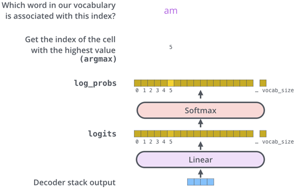
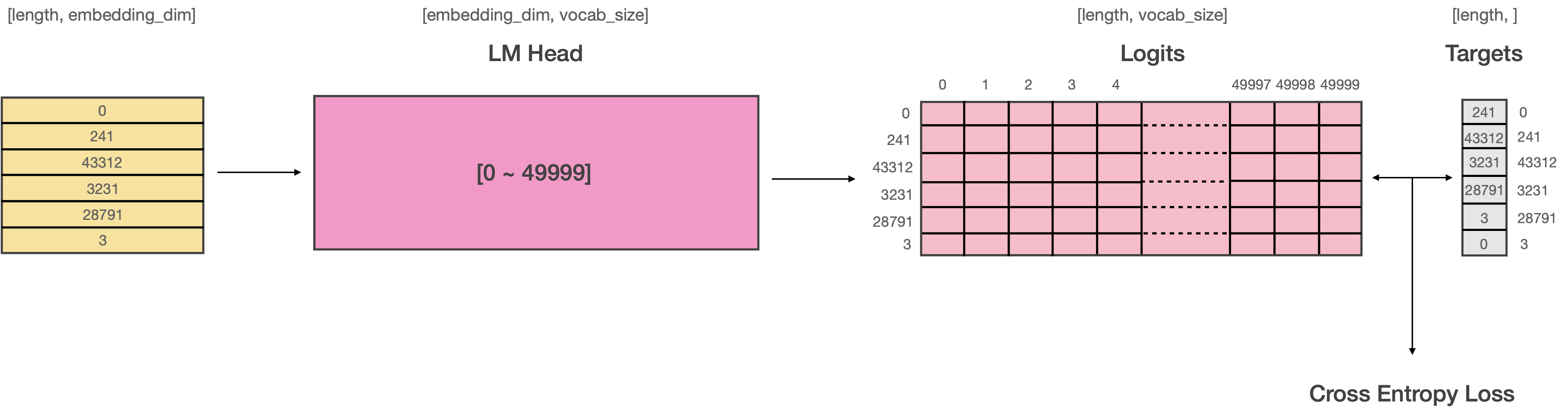
# 그러나 여기서 문제가 생깁니다. 일반적으로 LM Head로 부터 출력된 Logits과 Target 데이터 사이의 Loss를 계산할 때는 다음과 같은 과정이 일어납니다.
#
#
#
# 
#
#
#
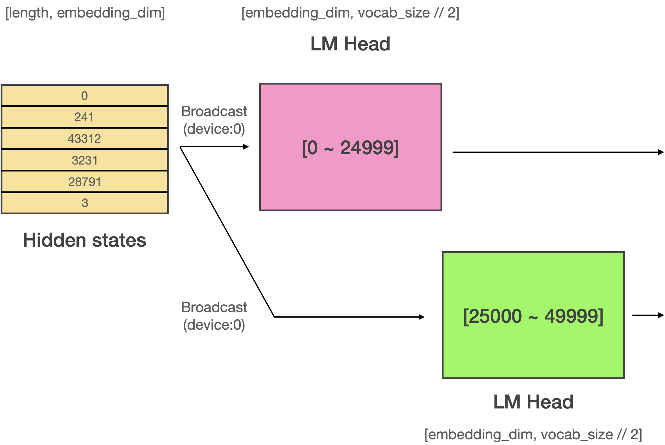
# 그러나 Megatron-LM은 Vocab Parallel Embedding을 사용하기 때문에 Embedding 레이어가 여러 디바이스를 걸쳐 분할되어 있습니다. 때문에 weight tying을 하게 된다면 **출력 임베딩(LM Head) 역시 여러 디바이스로 분할**되게 됩니다. 따라서 모델에서 출력되는 Logits의 사이즈는 vocab size를 분할한 사이즈가 됩니다.
#
#
#
# 
#
#
#
# 위 그림처럼 vocab size가 50,000이라면 원래는 (bsz, length, 50000)의 텐서가 출력되어야 하지만 위의 예시처럼 2개의 디바이스로 분할되어 있다면 (bsz, length, 25000)의 사이즈를 갖는 2개의 logits이 나오게 되며, 각 디바이스의 logits은 서로 다른 값을 갖게 될 것입니다. **이 것을 Parallel LM Logits이라고 부릅니다.** 이렇게 되면 target sentence와의 loss를 어떻게 계산해야 할까요? Traget 데이터에는 0번 부터 49999번째 토큰까지 모두 존재하는데 비해 logits의 사이즈는 그 절반밖에 되지 않으니까요.
#
#
#
# 
#
#
#
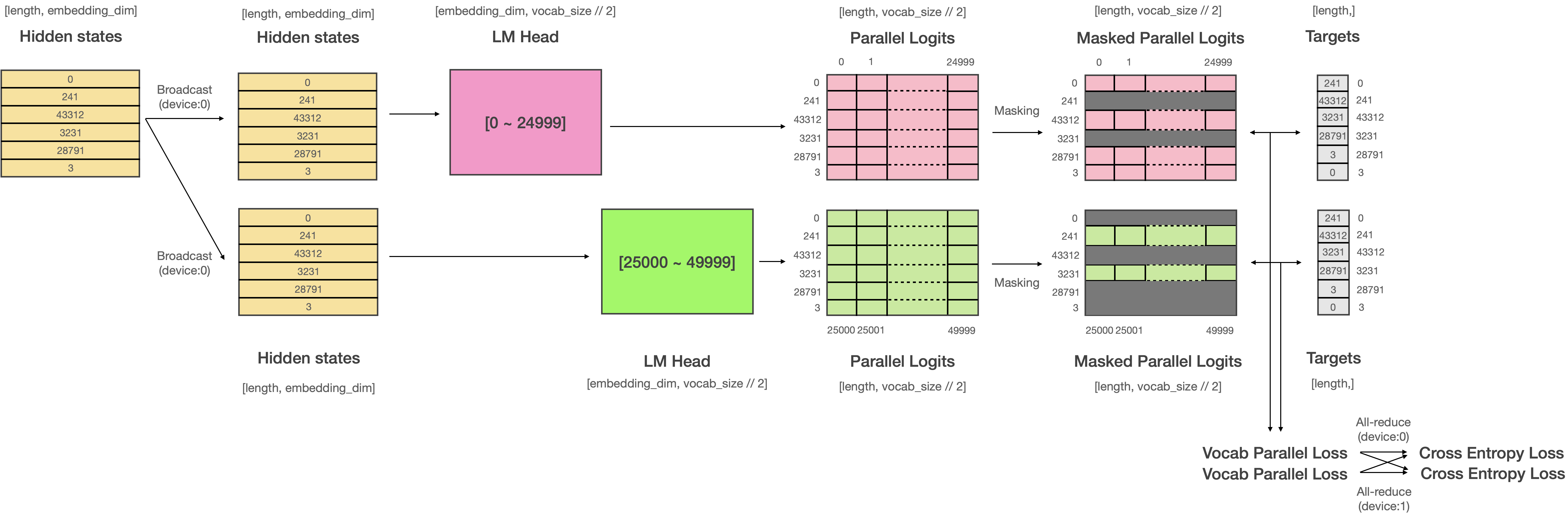
# 이 경우 **기존의 cross entropy가 아닌 vocab parallel cross entropy라고 불리는 특별한 loss 함수를 사용**해야 합니다. Vocab parallel corss entropy loss의 연산은 위와 같이 진행됩니다. 계산된 Logit에서 해당 디바이스가 커버 할 수 있는 부분만 남기고 Masking하여 Loss를 계산합니다. 그리고 계산된 Loss들을 All-reduce 해서 최종 Loss를 계산합니다.
# In[ ]:
"""
참고: _VocabParallelCrossEntropy in megatron-lm/megatron/mpu/cross_entropy.py
"""
@staticmethod
def forward(ctx, vocab_parallel_logits, target):
# Maximum value along vocab dimension across all GPUs.
logits_max = torch.max(vocab_parallel_logits, dim=-1)[0]
torch.distributed.all_reduce(logits_max,
op=torch.distributed.ReduceOp.MAX,
group=get_tensor_model_parallel_group())
# Subtract the maximum value.
vocab_parallel_logits.sub_(logits_max.unsqueeze(dim=-1))
# Get the partition's vocab indecies
get_vocab_range = VocabUtility.vocab_range_from_per_partition_vocab_size
partition_vocab_size = vocab_parallel_logits.size()[-1]
rank = get_tensor_model_parallel_rank()
world_size = get_tensor_model_parallel_world_size()
vocab_start_index, vocab_end_index = get_vocab_range(
partition_vocab_size, rank, world_size)
# Create a mask of valid vocab ids (1 means it needs to be masked).
target_mask = (target < vocab_start_index) | (target >= vocab_end_index)
masked_target = target.clone() - vocab_start_index
masked_target[target_mask] = 0
# Get predicted-logits = logits[target].
# For Simplicity, we convert logits to a 2-D tensor with size
# [*, partition-vocab-size] and target to a 1-D tensor of size [*].
logits_2d = vocab_parallel_logits.view(-1, partition_vocab_size)
masked_target_1d = masked_target.view(-1)
arange_1d = torch.arange(start=0, end=logits_2d.size()[0],
device=logits_2d.device)
predicted_logits_1d = logits_2d[arange_1d, masked_target_1d]
predicted_logits_1d = predicted_logits_1d.clone().contiguous()
predicted_logits = predicted_logits_1d.view_as(target)
predicted_logits[target_mask] = 0.0
# All reduce is needed to get the chunks from other GPUs.
torch.distributed.all_reduce(predicted_logits,
op=torch.distributed.ReduceOp.SUM,
group=get_tensor_model_parallel_group())
# Sum of exponential of logits along vocab dimension across all GPUs.
exp_logits = vocab_parallel_logits
torch.exp(vocab_parallel_logits, out=exp_logits)
sum_exp_logits = exp_logits.sum(dim=-1)
torch.distributed.all_reduce(sum_exp_logits,
op=torch.distributed.ReduceOp.SUM,
group=get_tensor_model_parallel_group())
# Loss = log(sum(exp(logits))) - predicted-logit.
loss = torch.log(sum_exp_logits) - predicted_logits
# Store softmax, target-mask and masked-target for backward pass.
exp_logits.div_(sum_exp_logits.unsqueeze(dim=-1))
ctx.save_for_backward(exp_logits, target_mask, masked_target_1d)
return loss
# ### Megatron-LM으로 모델 학습해보기
#
# Megatron-LM을 사용해서 모델을 학습해보도록 하겠습니다. Megaton-LM은 Hugging Face `transformers`와 같이 코드레벨로 사용하는 프레임워크가 아니라 이미 잘 짜여진 코드를 활용하여 모델을 만드는 데에 쓰입니다. 따라서 레포를 클론한 뒤에 진행하도록 하겠습니다.
# In[5]:
# git과 wget이 설치되어있지 않다면 아래 명령어를 통해 설치합니다.
get_ipython().system('apt update && apt install git wget -y')
# In[6]:
# Megatron-LM을 clone 합니다.
get_ipython().system('git clone https://github.com/NVIDIA/Megatron-LM')
# In[7]:
get_ipython().run_line_magic('cd', 'Megatron-LM')
# 이제 필요한 몇가지 패키지를 설치해보도록 하겠습니다. Megatron-LM에는 `nltk`로 데이터를 문장단위로 분할해서 전처리 하는 기능이 있습니다. 저는 지금 이 기능을 사용하진 않을것이지만 설치되어 있지 않으면 에러가 발생하기 때문에 `nltk`를 설치하겠습니다.
# In[8]:
get_ipython().system('pip install nltk')
# Megatron-LM은 `pybind11`와 `apex` 패키지도 사용합니다. 설치하도록 하겠습니다. (CUDA 컴파일이 꽤 오래 걸리니 느긋하게 기다려주세요.)
# In[9]:
get_ipython().system('pip install pybind11')
# In[ ]:
get_ipython().system('git clone https://github.com/NVIDIA/apex')
get_ipython().run_line_magic('cd', 'apex')
get_ipython().system('pip install -v --disable-pip-version-check --no-cache-dir --global-option="--cpp_ext" --global-option="--cuda_ext" ./')
get_ipython().run_line_magic('cd', '..')
# 이제 데이터셋을 만들어보도록 하겠습니다. Megatron-LM으로 모델을 Pre-training을 할 때는 `{"text": "샘플"}`과 같은 json 구조가 여러라인으로 구성된 간단한 구조의 jsonl 파일을 만들면 되고, Fine-tuning의 경우는 해당 태스크에 맞게 데이터셋을 구성해야 합니다. 본 튜토리얼에서는 Pre-training만 다루고 있기 때문에 Fine-tuning이 필요하시면 Megatron-LM 깃헙 레포를 참고해주세요.
# In[ ]:
"""
src/megatron_datasets.py
"""
import json
import os
from datasets import load_dataset
train_samples, min_length = 10000, 512
filename = "megatron_datasets.jsonl"
curr_num_datasets = 0
if os.path.exists(filename):
os.remove(filename)
datasets = load_dataset("wikitext", "wikitext-103-raw-v1")
datasets = datasets.data["train"]["text"]
dataset_fp_write = open(filename, mode="w", encoding="utf-8")
for sample in datasets:
sample = sample.as_py()
if len(sample) >= min_length:
line = json.dumps(
{"text": sample},
ensure_ascii=False,
)
dataset_fp_write.write(line + "\n")
curr_num_datasets += 1
# 튜토리얼이기 때문에 적은 양의 데이터만 만들겠습니다.
if curr_num_datasets >= train_samples:
break
dataset_fp_read = open(filename, mode="r", encoding="utf-8")
dataset_read = dataset_fp_read.read().splitlines()[:3]
# 데이터의 구조를 확인합니다.
for sample in dataset_read:
print(sample, end="\n\n")
# In[11]:
get_ipython().system('python ../../src/megatron_datasets.py')
# Tokenization에 사용할 Vocab을 다운로드 받습니다.
# In[12]:
get_ipython().system('wget https://huggingface.co/gpt2/raw/main/vocab.json')
get_ipython().system('wget https://huggingface.co/gpt2/raw/main/merges.txt')
# In[13]:
get_ipython().run_line_magic('ls', '')
# 이제 Dataset을 전처리합니다. 여기서 수행하는 전처리는 Tokenization과 Binarization을 함께 수행합니다. Megatron-LM의 전처리 코드는 Fairseq의 Indexed dataset의 코드를 카피해서 사용하고 있습니다. Fairseq의 데이터셋 전처리에 사용되는 방식은 크게 `lazy`, `cached`, `mmap` 등 크게 3가지가 존재하는데, 전처리 방식들에 대해 간략하게 설명하고 진행하겠습니다.
# #### 1) Lazy
# `lazy`는 필요한 데이터를 매 스텝마다 디스크에서 메모리로 불러옵니다. 즉, `Dataset` 클래스에서 `__getitem__()`이 호출 될 때마다 지정된 주소에 접근하여 데이터를 메모리로 로드하는 방식입니다. 그러나 매 스텝마다 File Buffer를 통해 디스크와의 I/O를 수행하기 때문에 처리 속도가 다소 느릴 수 있습니다.
# In[ ]:
"""
참고: fairseq/fairseq/data/indexed_dataset.py
주석은 제가 직접 추가하였습니다.
"""
from typing import Union
import numpy as np
def __getitem__(self, idx: Union[int, slice]) -> np.ndarray:
if not self.data_file:
# 파일 버퍼 로드
self.read_data(self.path)
if isinstance(idx, int):
# 인덱스 유효성 체크
self.check_index(idx)
# 로드할 텐서 사이즈 계산
tensor_size = self.sizes[self.dim_offsets[idx] : self.dim_offsets[idx + 1]]
# 텐서를 담을 빈 메모리 공간 할당
array = np.empty(tensor_size, dtype=self.dtype)
# offset을 기반으로 읽어올 파일의 디스크 주소를 지정
self.data_file.seek(self.data_offsets[idx] * self.element_size)
# 디스크로부터 메모리로 데이터 로드 (파일 I/O)
self.data_file.readinto(array)
return array
# #### 2) Cached
# `cached`는 모든 데이터를 학습 이전에 prefetch 하여 인메모리에 올려두고 접근하는 방식입니다. 학습 중에 데이터 로딩을 위해 디스크에 접근하지 않기 때문에 속도가 다른 방식들 보다는 빠른 편이지만 메모리의 크기에는 한계가 존재하므로 데이터셋의 용량이 매우 큰 경우에는 사용하기 어렵습니다.
#
# In[ ]:
"""
참고: fairseq/fairseq/data/indexed_dataset.py
주석은 제가 직접 추가하였습니다.
"""
from typing import List
def prefetch(self, indices: List[int]) -> None:
if all(i in self.cache_index for i in indices):
# 이미 모든 데이터가 캐싱되었다면 메서드 종료
return
if not self.data_file:
# 파일버퍼가 로드되지 않았다면 파일버퍼를 로드
self.read_data(self.path)
# 연속된 전체 메모리 사이즈를 계산하기 위해서 indices를 정렬
indices = sorted(set(indices))
total_size = 0
for i in indices:
total_size += self.data_offsets[i + 1] - self.data_offsets[i]
# 캐시로 사용할 전체 메모리 공간 할당
self.cache = np.empty(
total_size,
dtype=self.dtype,
)
self.cache_index.clear()
ptx = 0
for i in indices:
# 전체 어레이 사이즈를 저장
self.cache_index[i] = ptx
# offset으로부터 데이터 사이즈를 계산해서 현재 샘플이 저장될 메모리 공간을 변수에 할당
size = self.data_offsets[i + 1] - self.data_offsets[i]
array = self.cache[ptx : ptx + size]
# offset을 기반으로 읽어올 파일의 디스크 주소를 지정
self.data_file.seek(self.data_offsets[i] * self.element_size)
# 현재의 샘플을 할당된 메모리에 씀
self.data_file.readinto(array)
ptx += size
if self.data_file:
# 파일버퍼의 데이터를 모두 불러왔으니 버퍼를 닫고 참조를 해제
self.data_file.close()
self.data_file = None
# In[ ]:
"""
참고: fairseq/fairseq/data/indexed_dataset.py
주석은 제가 직접 추가하였습니다.
"""
def __getitem__(self, idx: Union[int, tuple]) -> Union[np.ndarray, List]:
if isinstance(idx, int):
# 인덱스 유효성 검사
self.check_index(idx)
# 텐서 사이즈 계산
tensor_size = self.sizes[self.dim_offsets[idx] : self.dim_offsets[idx + 1]]
# 메모리 공간 할당
array = np.empty(tensor_size, dtype=self.dtype)
# 프리패치된 데이터를 로드 (파일 I/O가 일어나지 않음)
ptx = self.cache_index[idx]
# 캐시에 프리패치된 데이터를 메모리 공간에 복사
np.copyto(array, self.cache[ptx : ptx + array.size])
return array
elif isinstance(idx, slice):
return [self[i] for i in range(*idx.indices(len(self)))]
# #### 3) Mmap
# `mmap`은 `lazy`와 동일하게 매 스텝마다 필요한 만큼의 데이터를 메모리로 로드하지만 File Buffer 대신 Memory Map을 사용하는 방식입니다. Memory Map은 File Buffer와 달리 현재 프로세스에게 할당된 가상메모리에 파일의 주소를 맵핑시키기 때문에 데이터가 마치 메모리 상에 존재하는 것 처럼 작업할 수 있습니다. 디스크와의 직접적인 I/O를 수행하지 않으며 페이지(4KB) 단위로 데이터를 로드 할 수 있고 실제로 메모리에서 모든 작업이 일어나기 때문에 File Buffer에 비해 처리 속도가 비교적 빠른 편입니다.
# In[ ]:
"""
참고: fairseq/fairseq/data/indexed_dataset.py
주석은 제가 직접 추가하였습니다.
"""
def __init__(self, path: str):
with open(path, "rb") as stream:
# 1. 매직 스트링 로드
# 매직스트링은 현재 저장된 데이터 구조가 어떤 형식인지 구분하기 위한 것.
# lazy인지 mmap인지 등등... (cached는 lazy와 같은 값을 가짐)
magic_test = stream.read(9)
assert magic_test == self._HDR_MAGIC, (
"Index file doesn't match expected format. "
"Please check your configuration file."
)
# 2. 버전 로드 (little endian unsigned long long)
# 코드 보니까 버전은 무조건 1로 쓰던데 별 의미 없는 변수인듯?
# b'\x01\x00\x00\x00\x00\x00\x00\x00'
version = struct.unpack(" np.ndarray:
if not self.data_file:
# 인덱스 파일이 로드되지 않았다면 로드
self.read_data(self.path)
if isinstance(idx, int):
# 인덱스 유효성 검사
self.check_index(idx)
# 텐서 사이즈 계산
tensor_size = self.sizes[self.dim_offsets[idx] : self.dim_offsets[idx + 1]]
# 메모리 공간 할당
array = np.empty(tensor_size, dtype=self.dtype)
# offset을 기반으로 읽어올 데이터의 가상메모리 주소를 지정
self.data_file.seek(self.data_offsets[idx] * self.element_size)
# 메모리로 데이터 로드
self.data_file.readinto(array)
return array
elif isinstance(idx, slice):
start, stop, step = idx.indices(len(self))
if step != 1:
# 슬라이스로 입력시 반드시 반드시 연속되어야 함
raise ValueError("Slices into indexed_dataset must be contiguous")
# 텐서의 사이즈들이 담긴 리스트와 전체 합을 계산
sizes = self.sizes[self.dim_offsets[start] : self.dim_offsets[stop]]
total_size = sum(sizes)
# 필요한 만큼의 메모리 공간 할당
array = np.empty(total_size, dtype=self.dtype)
# offset을 기반으로 읽어올 데이터의 가상메모리 주소를 지정
self.data_file.seek(self.data_offsets[start] * self.element_size)
self.data_file.readinto(array)
# 텐서 사이즈를 기반으로 여러개의 샘플로 분할
offsets = list(accumulate(sizes))
sentences = np.split(array, offsets[:-1])
return sentences
# 이제 데이터셋 전처리를 수행합니다. 저는 `mmap` 방식을 사용하여 전처리 하도록 하겠습니다.
#
# 이 때, `append-eod`라는 옵션이 보입니다. Megatron-LM은 패딩을 만들지 않기 위해 Pre-train 시에 모든 데이터를 연결해서 학습합니다. 예를 들어, `{"text": "I am a boy."}`"라는 샘플과 `{"text": "You are so lucky"}`라는 샘플이 있으면 Pre-train 할 때는 `input = "I am a boy. You are so lucky ..."`과 같이 모든 샘플을 연결합니다. 그리고나서 사용자가 설정한 길이(e.g. 2048)로 데이터를 잘라서 학습합니다.
#
# 그러나 이렇게 모든 샘플을 하나의 문자열로 연결해버리면 샘플과 샘플사이에 구분이 없어지기 때문에 문제가 될 수 있는데요. `append-eod` 옵션을 추가하면 샘플들 사이에 `end of document`로써 토큰을 추가하여 샘플과 샘플을 구분합니다. GPT2의 경우, `eod` 토큰은 `eos`토큰으로 설정되어 있습니다.
# In[14]:
get_ipython().system('python tools/preprocess_data.py --input megatron_datasets.jsonl --output-prefix my-gpt2 --vocab vocab.json --dataset-impl mmap --tokenizer-type GPT2BPETokenizer --merge-file merges.txt --append-eod')
# 데이터셋 전처리가 완료되었습니다. 데이터를 확인해봅시다.
#
# - my-gpt2_text_document.bin
# - my-gpt2_text_document.idx
#
# 와 같은 파일들이 생겼습니다. `idx`파일은 데이터의 위치 등의 메타데이터가 저장되어 있으며, `bin` 파일에는 실제로 Tokenized 된 데이터가 저장되어 있습니다.
# In[15]:
get_ipython().run_line_magic('ls', '')
# 이제 모델 학습을 시작해보겠습니다.
# In[16]:
# 일단 Tensor parallelism만 사용해보도록 하겠습니다.
# Data parallelism과 Pipeline parallelism은 Multi-dimensional Parallelism 세션에서 사용해봅시다. :)
# 학습은 1000 스텝만 시키도록 하겠습니다. 실제 학습할 땐 더 많은 숫자로 설정해주세요.
get_ipython().system('python -m torch.distributed.launch --nproc_per_node "4" --nnodes "1" --node_rank "0" --master_addr "localhost" --master_port "6000" ./pretrain_gpt.py --num-layers "24" --hidden-size "1024" --num-attention-heads "16" --seq-length "1024" --max-position-embeddings "1024" --micro-batch-size "4" --global-batch-size "8" --lr "0.00015" --train-iters "1000" --lr-decay-iters "300" --lr-decay-style cosine --vocab-file "vocab.json" --merge-file "merges.txt" --lr-warmup-fraction ".01" --fp16 --log-interval "10" --save-interval "500" --eval-interval "100" --eval-iters 10 --activations-checkpoint-method "uniform" --save "checkpoints/gpt2_345m" --load "checkpoints/gpt2_345m" --data-path "my-gpt2_text_document" --tensor-model-parallel-size "4" --pipeline-model-parallel-size "1" --DDP-impl "torch"')
# Megatron-LM에는 위에 설정한 옵션 이외에도 굉장히 많은 옵션들이 있습니다.
# 모든 옵션을 설명하기는 어려우니 아래 주소를 참고해주세요.
# https://github.com/NVIDIA/Megatron-LM/blob/main/megatron/arguments.py
# In[18]:
get_ipython().run_line_magic('cd', '..')
#
#
# ## 3. Parallelformers
#
#  #
# 지금까지 Megatron-LM으로 모델을 학습해봤습니다. Megatron-LM은 훌륭한 Tensor Parallelism 기능을 보유하고 있지만, 기존에 우리가 자주 쓰던 Hugging Face `transformers`로 학습된 모델을 병렬화 할 수는 없었습니다. 이러한 문제를 해결하기 위해 TUNiB은 2021년 `parallelformers`라는 오픈소스를 공개했습니다. `parallelformers`는 코드 한 두줄로 Hugging Face `transformers`로 학습된 거의 대부분의 모델에 Tensor Parallelism을 적용하여 인퍼런스 할 수 있는 도구 입니다.
#
# `parallelformers`를 설치해봅시다.
# In[19]:
get_ipython().system('pip install parallelformers')
# `parallelformers`는 아래 코드와 같이 `parallelize` 함수를 이용하여 기존 모델을 병렬화 할 수 있으며, `num_gpus`와 `fp16` 등의 몇가지 옵션을 추가로 제공합니다.
# In[ ]:
from transformers import AutoModelForCausalLM, AutoTokenizer
from parallelformers import parallelize
if __name__ == "__main__":
model = AutoModelForCausalLM.from_pretrained("EleutherAI/gpt-neo-2.7B")
tokenizer = AutoTokenizer.from_pretrained("EleutherAI/gpt-neo-2.7B")
parallelize(model, num_gpus=4, fp16=True, verbose="simple")
inputs = tokenizer(
"Parallelformers is",
return_tensors="pt",
)
outputs = model.generate(
**inputs,
num_beams=5,
no_repeat_ngram_size=4,
max_length=15,
)
print(f"\nOutput: {tokenizer.batch_decode(outputs)[0]}")
# 주의: `parallelformers`는 프로세스간 데이터 통신을 위해 공유메모리를 사용합니다. 따라서 **docker와 같이 제한된 리소스만 허용되는 환경에서 사용할 때는 반드시 shared memory 사이즈를 키워줘야 합니다.**
#
# `docker run ... --shm_size=?gb` 옵션을 통해 공유메모리 사이즈를 키우거나 `docker run ... --ipc=host` 옵션을 통해 공유메모리 제한을 해제할 수 있습니다. docker에서 발생하는 거의 모든 문제는 공유메모리의 제한 때문에 일어나는 것으로 확인 되었으며 더 큰 모델을 사용하려면 더 큰 사이즈의 shared memory 할당이 요구됩니다.
# In[20]:
get_ipython().system('python ../src/parallelformers_inference.py')
# ### Parallelformers의 동작 원리
#
#
#
# 
#
#
#
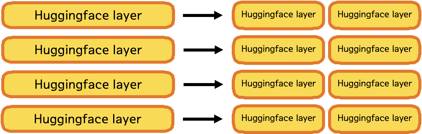
# 그렇다면 `parallelformers`는 어떻게 모델링 코드의 변화 없이 Tensor parallelism을 수행 할 수 있을까요? 정답은 `Tensor Replacement` 메커니즘에 있습니다. `parallelformers`는 기존 모델의 파라미터를 전부 추출한 뒤, Megatron-LM과 동일한 방식으로 텐서를 쪼개고 쪼개진 텐서로 원래 모델에 존재하던 파라미터를 교체함으로써 모델의 구조 변화 없이 병렬화를 수행할 수 있었습니다. 이를 통해 약 70여가지의 모델을 병렬화 할 수 있었습니다. 이외에도 몇가지 메커니즘이 도입되었지만 텐서 병렬화와 관계 있는 내용은 아니기 때문에 생략하도록 하겠습니다. 만약 더 자세한 내용이 궁금하시다면 다음 주소를 참고해주세요.
#
# - 한국어: https://tunib.notion.site/TECH-2021-07-26-Parallelformers-_-0dcceeaddc5247429745ba36c6549fe5
# - English: https://tunib.notion.site/TECH-2021-07-26-Parallelformers-Journey-to-deploying-big-models_TUNiB-32b19a599c38497abaad2a98727f6dc8