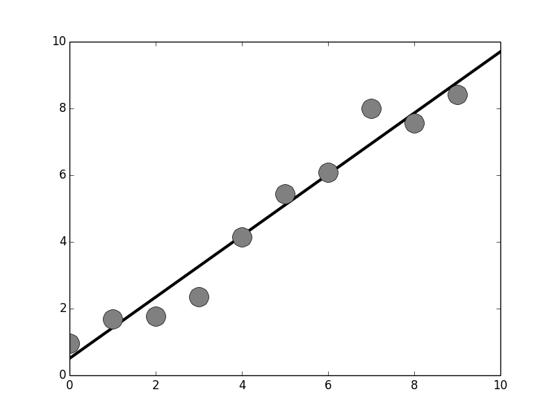
The Scikit-learn module can easily perform basic linear regression. The circles show the training data and the fitted line is shown in black.
# #
#
#
#
#
# **Multilinear Regression.** The Scikit-learn module easily extends
# linear regression to multiple dimensions. For example, for
# multi-linear regression,
# $$
# y = \alpha_0 + \alpha_1 x_1 + \alpha_2 x_2 + \ldots + \alpha_n x_n
# $$
# The problem is to find all of the $\alpha$ terms given the
# training set $\left\{x_1,x_2,\ldots,x_n,y\right\}$. We can create another
# example data set and see how this works,
# In[8]:
X=np.random.randint(20,size=(10,2))
Y=X.dot([1,3])+1 + np.random.randn(X.shape[0])*20
# In[9]:
ym=Y/Y.max() # scale for marker size
fig,ax=subplots()
_=ax.scatter(X[:,0],X[:,1],ym*400,color='gray',alpha=.7,label=r'$Y=f(X_1,X_2)$')
_=ax.set_xlabel(r'$X_1$',fontsize=22)
_=ax.set_ylabel(r'$X_2$',fontsize=22)
_=ax.set_title('Two dimensional regression',fontsize=20)
_=ax.legend(loc=4,fontsize=22)
fig.tight_layout()
fig.savefig('fig-machine_learning/python_machine_learning_modules_003.png')
#
#
#
#
#
#
#
#
#
#
# **Multilinear Regression.** The Scikit-learn module easily extends
# linear regression to multiple dimensions. For example, for
# multi-linear regression,
# $$
# y = \alpha_0 + \alpha_1 x_1 + \alpha_2 x_2 + \ldots + \alpha_n x_n
# $$
# The problem is to find all of the $\alpha$ terms given the
# training set $\left\{x_1,x_2,\ldots,x_n,y\right\}$. We can create another
# example data set and see how this works,
# In[8]:
X=np.random.randint(20,size=(10,2))
Y=X.dot([1,3])+1 + np.random.randn(X.shape[0])*20
# In[9]:
ym=Y/Y.max() # scale for marker size
fig,ax=subplots()
_=ax.scatter(X[:,0],X[:,1],ym*400,color='gray',alpha=.7,label=r'$Y=f(X_1,X_2)$')
_=ax.set_xlabel(r'$X_1$',fontsize=22)
_=ax.set_ylabel(r'$X_2$',fontsize=22)
_=ax.set_title('Two dimensional regression',fontsize=20)
_=ax.legend(loc=4,fontsize=22)
fig.tight_layout()
fig.savefig('fig-machine_learning/python_machine_learning_modules_003.png')
#
#
#
#
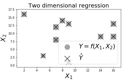
# Scikit-learn can easily perform multi-linear regression. The size of the circles indicate the value of the two-dimensional function of $(X_1,X_2)$.
# #
#
#
#
# [Figure](#fig:python_machine_learning_modules_003) shows the
# two dimensional regression example, where the size of the circles is
# proportional to the targetted $Y$ value. Note that we salted the output
# with random noise just to keep things interesting. Nonetheless, the
# interface with Scikit-learn is the same,
# In[10]:
lr=LinearRegression()
lr.fit(X,Y)
print(lr.coef_)
# The `coef_` variable now has two terms in it,
# corresponding to the two input dimensions. Note that the constant
# offset is already built-in and is an option on the `LinearRegression`
# constructor. [Figure](#fig:python_machine_learning_modules_004) shows
# how the regression performs.
# In[11]:
_=lr.fit(X,Y)
yp=lr.predict(X)
ypm=yp/yp.max() # scale for marker size
_=ax.scatter(X[:,0],X[:,1],ypm*400,marker='x',color='k',lw=2,alpha=.7,label=r'$\hat{Y}$')
_=ax.legend(loc=0,fontsize=22)
_=fig.canvas.draw()
fig.savefig('fig-machine_learning/python_machine_learning_modules_004.png')
#
#
#
#
#
#
#
#
#
# [Figure](#fig:python_machine_learning_modules_003) shows the
# two dimensional regression example, where the size of the circles is
# proportional to the targetted $Y$ value. Note that we salted the output
# with random noise just to keep things interesting. Nonetheless, the
# interface with Scikit-learn is the same,
# In[10]:
lr=LinearRegression()
lr.fit(X,Y)
print(lr.coef_)
# The `coef_` variable now has two terms in it,
# corresponding to the two input dimensions. Note that the constant
# offset is already built-in and is an option on the `LinearRegression`
# constructor. [Figure](#fig:python_machine_learning_modules_004) shows
# how the regression performs.
# In[11]:
_=lr.fit(X,Y)
yp=lr.predict(X)
ypm=yp/yp.max() # scale for marker size
_=ax.scatter(X[:,0],X[:,1],ypm*400,marker='x',color='k',lw=2,alpha=.7,label=r'$\hat{Y}$')
_=ax.legend(loc=0,fontsize=22)
_=fig.canvas.draw()
fig.savefig('fig-machine_learning/python_machine_learning_modules_004.png')
#
#
#
#
# The predicted data is plotted in black. It overlays the training data, indicating a good fit.
# #
#
#
#
#
# **Polynomial Regression.** We can extend this to include polynomial
# regression by using the `PolynomialFeatures` in the `preprocessing`
# sub-module. To keep it simple, let's go back to our one-dimensional
# example. First, let's create some synthetic data,
# In[12]:
from sklearn.preprocessing import PolynomialFeatures
X = np.arange(10).reshape(-1,1) # create some data
Y = X+X**2+X**3+ np.random.randn(*X.shape)*80
#
#
# Next, we have to create a transformation
# from `X` to a polynomial of `X`,
# In[13]:
qfit = PolynomialFeatures(degree=2) # quadratic
Xq = qfit.fit_transform(X)
print(Xq)
# Note there is an automatic constant term in the output $0^{th}$
# column where `fit_transform` has mapped the single-column input into a set of
# columns representing the individual polynomial terms. The middle column has
# the linear term, and the last has the quadratic term. With these polynomial
# features stacked as columns of `Xq`, all we have to do is `fit` and `predict`
# again. The following draws a comparison between the linear regression and the
# quadratic regression (see [Figure](#fig:python_machine_learning_modules_005)),
# In[14]:
lr=LinearRegression() # create linear model
qr=LinearRegression() # create quadratic model
lr.fit(X,Y) # fit linear model
qr.fit(Xq,Y) # fit quadratic model
lp = lr.predict(xi)
qp = qr.predict(qfit.fit_transform(xi))
#
#
#
#
#
#
#
#
#
#
# **Polynomial Regression.** We can extend this to include polynomial
# regression by using the `PolynomialFeatures` in the `preprocessing`
# sub-module. To keep it simple, let's go back to our one-dimensional
# example. First, let's create some synthetic data,
# In[12]:
from sklearn.preprocessing import PolynomialFeatures
X = np.arange(10).reshape(-1,1) # create some data
Y = X+X**2+X**3+ np.random.randn(*X.shape)*80
#
#
# Next, we have to create a transformation
# from `X` to a polynomial of `X`,
# In[13]:
qfit = PolynomialFeatures(degree=2) # quadratic
Xq = qfit.fit_transform(X)
print(Xq)
# Note there is an automatic constant term in the output $0^{th}$
# column where `fit_transform` has mapped the single-column input into a set of
# columns representing the individual polynomial terms. The middle column has
# the linear term, and the last has the quadratic term. With these polynomial
# features stacked as columns of `Xq`, all we have to do is `fit` and `predict`
# again. The following draws a comparison between the linear regression and the
# quadratic regression (see [Figure](#fig:python_machine_learning_modules_005)),
# In[14]:
lr=LinearRegression() # create linear model
qr=LinearRegression() # create quadratic model
lr.fit(X,Y) # fit linear model
qr.fit(Xq,Y) # fit quadratic model
lp = lr.predict(xi)
qp = qr.predict(qfit.fit_transform(xi))
#
#
#
#
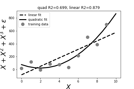
# The title shows the $R^2$ score for the linear and quadratic rogressions.
# #
#
# In[15]:
fig,ax=subplots()
_=ax.plot(xi,lp,'--k',lw=3,label='linear fit')
_=ax.plot(xi,qp,'-k',lw=3,label='quadratic fit')
_=ax.plot(X.flat,Y.flat,'o',color='gray',ms=10,label='training data')
_=ax.legend(loc=0)
_=ax.set_title('quad R2={:.3}; linear R2={:.3}'.format(lr.score(X,Y),qr.score(Xq,Y)))
_=ax.set_xlabel('$X$',fontsize=22)
_=ax.set_ylabel(r'$X+X^2+X^3+\epsilon$',fontsize=22)
fig.savefig('fig-machine_learning/python_machine_learning_modules_005.png')
# This just scratches the surface of Scikit-learn. We will go through
# many more examples later, but the main thing is to concentrate on the
# usage (i.e., `fit`, `predict`) which is standardized across all of the
# machine learning methods in Scikit-learn.
#
#
# In[15]:
fig,ax=subplots()
_=ax.plot(xi,lp,'--k',lw=3,label='linear fit')
_=ax.plot(xi,qp,'-k',lw=3,label='quadratic fit')
_=ax.plot(X.flat,Y.flat,'o',color='gray',ms=10,label='training data')
_=ax.legend(loc=0)
_=ax.set_title('quad R2={:.3}; linear R2={:.3}'.format(lr.score(X,Y),qr.score(Xq,Y)))
_=ax.set_xlabel('$X$',fontsize=22)
_=ax.set_ylabel(r'$X+X^2+X^3+\epsilon$',fontsize=22)
fig.savefig('fig-machine_learning/python_machine_learning_modules_005.png')
# This just scratches the surface of Scikit-learn. We will go through
# many more examples later, but the main thing is to concentrate on the
# usage (i.e., `fit`, `predict`) which is standardized across all of the
# machine learning methods in Scikit-learn.