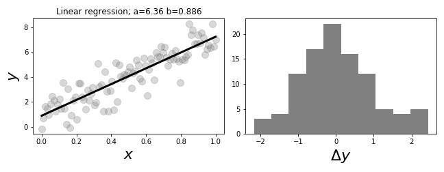
The panel on the left # shows the data and regression line. The panel on the right shows a histogram of # the regression errors.
# #
#
#
#
# The graph on the left of
# [Figure](#fig:Regression_001)
# shows the regression line plotted against the
# data. The estimated
# parameters are noted in the title. The histogram on the
# right of
# [Figure](#fig:Regression_001) shows the residual errors in the model.
# It is always a good idea to inspect the residuals of any regression
# for
# normality. These are the differences between the fitted line for
# each $x_i$
# value and the corresponding $y_i$ value in the data.
# Note that the $x$ term does
# not have to be uniformly monotone.
#
# To decouple the deterministic variation from
# the random variation, we can fix
# the index and write separate problems of the
# form
#
# $$
# y_i = a x_i +b + \epsilon_i
# $$
#
# where $\epsilon_i \sim \mathcal{N}(0,\sigma^2)$. What could we do with
# just
# this one component of the problem? In other words, suppose we had
# $m$-samples of
# this component as in $\lbrace y_{i,k}\rbrace_{k=1}^m$. Following
# the usual
# procedure, we could obtain estimates of the mean of $y_i$ as
#
# $$
# \hat{y_i} = \frac{1}{m}\sum_{k=1}^m y_{i,k}
# $$
#
# However, this tells us nothing about the individual parameters $a$
# and $b$
# because they are not separable in the terms that are computed, namely,
# we may
# have
#
# $$
# \mathbb{E}(y_i) = a x_i +b
# $$
#
# but we still only have one equation and the two unknowns, $a$ and
# $b$. How
# about if we consider and fix another component $j$ as in
#
# $$
# y_j = a x_j +b + \epsilon_i
# $$
#
# Then, we have
#
# $$
# \mathbb{E}(y_j) = a x_j +b
# $$
#
# so at least now we have two equations and two unknowns and we know how to
# estimate the left hand sides of these equations from the data using the
# estimators $\hat{y_i}$ and $\hat{y_j}$. Let's see how this works in the code
# sample below.
# In[4]:
x0, xn =x[0],x[80]
# generate synthetic data
y_0 = a*x0 + np.random.randn(20)+b
y_1 = a*xn + np.random.randn(20)+b
# mean along sample dimension
yhat = np.array([y_0,y_1]).mean(axis=1)
a_,b_=np.linalg.solve(np.array([[x0,1],
[xn,1]]),yhat)
#
#
#
#
#
#
#
#
#
# The graph on the left of
# [Figure](#fig:Regression_001)
# shows the regression line plotted against the
# data. The estimated
# parameters are noted in the title. The histogram on the
# right of
# [Figure](#fig:Regression_001) shows the residual errors in the model.
# It is always a good idea to inspect the residuals of any regression
# for
# normality. These are the differences between the fitted line for
# each $x_i$
# value and the corresponding $y_i$ value in the data.
# Note that the $x$ term does
# not have to be uniformly monotone.
#
# To decouple the deterministic variation from
# the random variation, we can fix
# the index and write separate problems of the
# form
#
# $$
# y_i = a x_i +b + \epsilon_i
# $$
#
# where $\epsilon_i \sim \mathcal{N}(0,\sigma^2)$. What could we do with
# just
# this one component of the problem? In other words, suppose we had
# $m$-samples of
# this component as in $\lbrace y_{i,k}\rbrace_{k=1}^m$. Following
# the usual
# procedure, we could obtain estimates of the mean of $y_i$ as
#
# $$
# \hat{y_i} = \frac{1}{m}\sum_{k=1}^m y_{i,k}
# $$
#
# However, this tells us nothing about the individual parameters $a$
# and $b$
# because they are not separable in the terms that are computed, namely,
# we may
# have
#
# $$
# \mathbb{E}(y_i) = a x_i +b
# $$
#
# but we still only have one equation and the two unknowns, $a$ and
# $b$. How
# about if we consider and fix another component $j$ as in
#
# $$
# y_j = a x_j +b + \epsilon_i
# $$
#
# Then, we have
#
# $$
# \mathbb{E}(y_j) = a x_j +b
# $$
#
# so at least now we have two equations and two unknowns and we know how to
# estimate the left hand sides of these equations from the data using the
# estimators $\hat{y_i}$ and $\hat{y_j}$. Let's see how this works in the code
# sample below.
# In[4]:
x0, xn =x[0],x[80]
# generate synthetic data
y_0 = a*x0 + np.random.randn(20)+b
y_1 = a*xn + np.random.randn(20)+b
# mean along sample dimension
yhat = np.array([y_0,y_1]).mean(axis=1)
a_,b_=np.linalg.solve(np.array([[x0,1],
[xn,1]]),yhat)
#
#
#
#
# The fitted and true lines are plotted with # the data values. The squares at either end of the solid line show the mean value # for each of the data groups shown.
# #
#
#
#
# **Programming
# Tip.**
#
# The prior code uses the `solve` function in the Numpy `linalg` module,
# which
# contains the core linear algebra codes in Numpy that incorporate the
# battle-tested LAPACK library.
#
#
#
# We can write out the solution for the
# estimated parameters for this
# case where $x_0 =0$
#
# $$
# \begin{align*}
# \hat{a} &= \frac{\hat{y}_i - \hat{y}_0}{x_i} \\\
# \hat{b} &=
# \hat{y_0} \\\
# \end{align*}
# $$
#
# The expectations and variances of these estimators are the following,
#
# $$
# \begin{align*}
# \mathbb{E}(\hat{a}) &= \frac{a x_i }{x_i}=a \\\
# \mathbb{E}(\hat{b}) &=b \\\
# \mathbb{V}(\hat{a}) &= \frac{2 \sigma^2}{x_i^2} \\\
# \mathbb{V}(\hat{b}) &= \sigma^2
# \end{align*}
# $$
#
# The expectations show that the estimators are unbiased. The
# estimator
# $\hat{a}$ has a variance that decreases as larger points $x_i$ are
# selected.
# That is, it is better to have samples further out along the
# horizontal axis for
# fitting the line. This variance quantifies the *leverage*
# of those distant
# points.
#
# **Regression From Projection Methods.** Let's see if we can apply our
# knowledge
# of projection methods to the general case. In vector notation, we can
# write
# the following:
#
# $$
# \mathbf{y} = a \mathbf{x} + b\mathbf{1} + \boldsymbol{\epsilon}
# $$
#
# where $\mathbf{1}$ is the vector of all ones.
# Let's use the inner-product
# notation,
#
# $$
# \langle \mathbf{x},\mathbf{y} \rangle = \mathbb{E}(\mathbf{x}^T \mathbf{y})
# $$
#
# Then, by taking the inner-product with some $\mathbf{x}_1 \in
# \mathbf{1}^\perp$
# we obtain [^perp],
#
# [^perp]: The space of all vectors, $\mathbf{a}$ such that
# $\langle
# \mathbf{a},\mathbf{1} \rangle = 0$ is denoted $\mathbf{1}^\perp$.
#
# $$
# \langle \mathbf{y},\mathbf{x}_1 \rangle = a \langle \mathbf{x},\mathbf{x}_1
# \rangle
# $$
#
# Recall that $\mathbb{E}(\boldsymbol{\epsilon})=\mathbf{0}$. We
# can finally
# solve for $a$ as
#
#
#
#
# $$
# \begin{equation}
# \hat{a} = \frac{\langle\mathbf{y},\mathbf{x}_1 \rangle}{\langle
# \mathbf{x},\mathbf{x}_1 \rangle}
# \end{equation}
# \label{eq:ahat} \tag{1}
# $$
#
# That was pretty neat but now we have the mysterious $\mathbf{x}_1$
# vector.
# Where does this come from? If we project $\mathbf{x}$ onto the
# $\mathbf{1}^\perp$, then we get the MMSE approximation to $\mathbf{x}$ in the
# $\mathbf{1}^\perp$ space. Thus, we take
#
# $$
# \mathbf{x}_1 = P_{\mathbf{1}^\perp} (\mathbf{x})
# $$
#
# Remember that $P_{\mathbf{1}^\perp} $ is a projection matrix so the length of
# $\mathbf{x}_1$ is at most $\mathbf{x}$. This means that the denominator in
# the
# $\hat{a}$ equation above is really just the length of the $\mathbf{x}$
# vector in
# the coordinate system of $P_{\mathbf{1}^\perp} $. Because the
# projection is
# orthogonal (namely, of minimum length), the Pythagorean theorem
# gives this
# length as the following:
#
# $$
# \langle \mathbf{x},\mathbf{x}_1 \rangle ^2=\langle \mathbf{x},\mathbf{x}
# \rangle- \langle\mathbf{1},\mathbf{x} \rangle^2
# $$
#
# The first term on the right is the length of the $\mathbf{x}$ vector
# and last
# term is the length of $\mathbf{x}$ in the coordinate system orthogonal
# to
# $P_{\mathbf{1}^\perp} $, namely that of $\mathbf{1}$. We
# can use this geometric
# interpretation to understand what is going on in
# typical linear regression in
# much more detail. The fact that the denominator is
# the orthogonal projection of
# $\mathbf{x}$ tells us that the choice of
# $\mathbf{x}_1$ has the strongest effect
# (i.e., largest value) on reducing
# the variance of $\hat{a}$. That is, the more
# $\mathbf{x}$ is aligned with
# $\mathbf{1}$, the worse the variance of $\hat{a}$.
# This makes intuitive sense
# because the closer $\mathbf{x}$ is to $\mathbf{1}$,
# the more constant it is,
# and we have already seen from our one-dimensional
# example that distance between
# the $x$ terms pays off in reduced variance. We
# already know that $\hat{a}$
# is an unbiased estimator, and, because we chose
# $\mathbf{x}_1$ deliberately as a
# projection, we know that it is also of minimum
# variance. Such estimators are
# known as Minimum-Variance Unbiased Estimators
# (MVUE).
#
# In the same spirit, let's examine the numerator of $\hat{a}$ in
# Equation [1](#eq:ahat). We can write
# $\mathbf{x}_{1}$ as the following
#
# $$
# \mathbf{x}_{1} = \mathbf{x} - P_{\mathbf{1}} \mathbf{x}
# $$
#
# where $P_{\mathbf{1}}$ is projection matrix of $\mathbf{x}$ onto the
# $\mathbf{1}$ vector. Using this, the numerator of $\hat{a}$ becomes
#
# $$
# \langle \mathbf{y}, \mathbf{x}_1\rangle =\langle \mathbf{y},
# \mathbf{x}\rangle -\langle \mathbf{y}, P_{\mathbf{1}} \mathbf{x}\rangle
# $$
#
# Note that,
#
# $$
# P_{\mathbf{1}} = \mathbf{1} \mathbf{1}^T \frac{1}{n}
# $$
#
# so that writing this out explicitly gives
#
# $$
# \langle \mathbf{y}, P_{\mathbf{1}} \mathbf{x}\rangle = \left(\mathbf{y}^T
# \mathbf{1}\right) \left(\mathbf{1}^T \mathbf{x}\right)/n =\left(\sum
# y_i\right)\left(\sum x_{i}\right)/n
# $$
#
# and similarly, we have the following for the denominator:
#
# $$
# \langle \mathbf{x}, P_{\mathbf{1}} \mathbf{x}\rangle = \left(\mathbf{x}^T
# \mathbf{1}\right) \left(\mathbf{1}^T \mathbf{x}\right)/n =\left(\sum
# x_i\right)\left(\sum x_{i}\right)/n
# $$
#
# So, plugging all of this together gives the following,
#
# $$
# \hat{a} = \frac{\mathbf{x}^T\mathbf{y}-(\sum x_i)(\sum y_i)/n}{\mathbf{x}^T
# \mathbf{x} -(\sum x_i)^2/n}
# $$
#
# with corresponding variance,
#
# $$
# \begin{align*}
# \mathbb{V}(\hat{a}) &= \sigma^2
# \frac{\|\mathbf{x}_1\|^2}{\langle\mathbf{x},\mathbf{x}_1\rangle^2} \\\
# &= \frac{\sigma^2}{\Vert \mathbf{x}\Vert^2-n(\overline{x}^2)}
# \end{align*}
# $$
#
# Using the same approach with $\hat{b}$ gives,
#
#
#
#
# $$
# \begin{equation}
# \hat{b} = \frac{\langle \mathbf{y},\mathbf{x}^{\perp}
# \rangle}{\langle \mathbf{1},\mathbf{x}^{\perp}\rangle}
# \label{_auto1} \tag{2}
# \end{equation}
# $$
#
#
#
#
# $$
# \begin{equation} \
# = \frac{\langle
# \mathbf{y},\mathbf{1}-P_{\mathbf{x}}(\mathbf{1})\rangle}{\langle
# \mathbf{1},\mathbf{1}-P_{\mathbf{x}}(\mathbf{1})\rangle}
# \label{_auto2} \tag{3}
# \end{equation}
# $$
#
#
#
#
# $$
# \begin{equation} \
# = \frac{\mathbf{x}^T \mathbf{x}(\sum y_i)/n
# -\mathbf{x}^T\mathbf{y}(\sum x_i)/n}{\mathbf{x}^T \mathbf{x} -(\sum x_i)^2/n}
# \label{_auto3} \tag{4}
# \end{equation}
# $$
#
# where
#
# $$
# P_{\mathbf{x}} = \frac{\mathbf{\mathbf{x} \mathbf{x}^T}}{\| \mathbf{x} \|^2}
# $$
#
# with variance
#
# $$
# \begin{align*}
# \mathbb{V}(\hat{b})&=\sigma^2 \frac{\langle
# \boldsymbol{\mathbf{1}-P_{\mathbf{x}}(\mathbf{1})},\boldsymbol{\mathbf{1}-P_{\mathbf{x}}(\mathbf{1})}\rangle}{\langle
# \mathbf{1},\boldsymbol{\mathbf{1}-P_{\mathbf{x}}(\mathbf{1})}\rangle^2} \\\
# &=\frac{\sigma^2}{n-\frac{(n\overline{x})^2}{\Vert\mathbf{x}\Vert^2}}
# \end{align*}
# $$
#
# **Qualifying the Estimates.** Our formulas for the variance above include the
# unknown $\sigma^2$, which we must estimate from the data itself using our
# plug-
# in estimates. We can form the residual sum of squares as
#
# $$
# \texttt{RSS} = \sum_i (\hat{a} x_i + \hat{b} - y_i)^2
# $$
#
# Thus, the estimate of $\sigma^2$ can be expressed as
#
# $$
# \hat{\sigma}^2 = \frac{\texttt{RSS}}{n-2}
# $$
#
# where $n$ is the number of samples. This is also known as the
# *residual mean
# square*. The $n-2$ represents the *degrees of freedom* (`df`).
# Because we
# estimated two parameters from the same data we have $n-2$ instead of
# $n$. Thus,
# in general, $\texttt{df} = n - p$, where $p$ is the number of
# estimated
# parameters. Under the assumption that the noise is Gaussian, the
# $\texttt{RSS}/\sigma^2$ is chi-squared distributed with $n-2$ degrees of
# freedom. Another important term is the *sum of squares about the mean*, (a.k.a
# *corrected* sum of squares),
#
# $$
# \texttt{SYY} = \sum (y_i - \bar{y})^2
# $$
#
# The $\texttt{SYY}$ captures the idea of not using the $x_i$ data and
# just using
# the mean of the $y_i$ data to estimate $y$. These two terms lead
# to the $R^2$
# term,
#
# $$
# R^2=1-\frac{\texttt{RSS}}{ \texttt{SYY} }
# $$
#
# Note that for perfect regression, $R^2=1$. That is, if the
# regression gets
# each $y_i$ data point exactly right, then
# $\texttt{RSS}=0$ this term equals one.
# Thus, this term is used to
# measure of goodness-of-fit. The `stats` module in
# `scipy` computes
# many of these terms automatically,
# In[5]:
from scipy import stats
slope,intercept,r_value,p_value,stderr = stats.linregress(x,y)
# where the square of the `r_value` variable is the $R^2$ above. The
# computed
# p-value is the two-sided hypothesis test with a null hypothesis that
# the slope
# of the line is zero. In other words, this tests whether or not the
# linear
# regression makes sense for the data for that hypothesis. The
# Statsmodels
# module provides a powerful extension to Scipy's stats module by
# making it easy
# to do regression and keep track of these parameters. Let's
# reformulate our
# problem using the Statsmodels framework by creating
# a Pandas dataframe for the
# data,
# In[6]:
import statsmodels.formula.api as smf
from pandas import DataFrame
import numpy as np
d = DataFrame({'x':np.linspace(0,1,10)}) # create data
d['y'] = a*d.x+ b + np.random.randn(*d.x.shape)
#
#
# Now that we have the input data in the above
# Pandas dataframe, we
# can perform the regression as in the following,
# In[7]:
results = smf.ols('y ~ x', data=d).fit()
# The $\sim$ symbol is notation for $y = a x + b + \epsilon$, where the
# constant
# $b$ is implicit in this usage of Statsmodels. The names in the string
# are taken
# from the columns in the dataframe. This makes it very easy to build
# models with
# complicated interactions between the named columns in the
# dataframe. We can
# examine a report of the model fit by looking at the summary,
# In[8]:
print (results.summary2())
# ```
#
# Results: Ordinary least squares
# =================================================================
# Model: OLS Adj. R-squared: 0.808
# Dependent Variable: y AIC: 28.1821
# Date: 0000-00-00 00:00 BIC: 00.0000
# No. Observations: 10 Log-Likelihood: -12.091
# Df Model: 1 F-statistic: 38.86
# Df Residuals: 8 Prob (F-statistic): 0.000250
# R-squared: 0.829 Scale: 0.82158
# -------------------------------------------------------------------
# Coef. Std.Err. t P>|t| [0.025 0.975]
# -------------------------------------------------------------------
# Intercept 1.5352 0.5327 2.8817 0.0205 0.3067 2.7637
# x 5.5990 0.8981 6.2340 0.0003 3.5279 7.6701
#
# There is a lot more here than we have discussed so far, but the
# Statsmodels
# documentation is the best place to go for complete information
# about this
# report. The F-statistic attempts to capture the contrast between
# including the
# slope parameter or leaving it off. That is, consider two
# hypotheses:
# ```
#
# $$
# \begin{align*}
# H_0 \colon \mathbb{E}(Y|X=x) &= b \\\
# H_1 \colon
# \mathbb{E}(Y|X=x) &= b + a x
# \end{align*}
# $$
#
# In order to quantify how much better adding the slope term is for
# the
# regression, we compute the following:
#
# $$
# F = \frac{\texttt{SYY} - \texttt{RSS}}{ \hat{\sigma}^2 }
# $$
#
# The numerator computes the difference in the residual squared errors
# between
# including the slope in the regression or just using the mean of the
# $y_i$
# values. Once again, if we assume (or can claim asymptotically) that the
# $\epsilon$ noise term is Gaussian, $\epsilon \sim \mathcal{N}(0,\sigma^2)$,
# then
# the $H_0$ hypothesis will follow an F-distribution [^fdist] with degrees of
# freedom from the numerator and denominator. In this case, $F \sim F(1,n-2)$.
# The
# value of this statistic is reported by Statsmodels above. The corresponding
# reported probability shows the chance of $F$ exceeding its computed value if
# $H_0$ were true. So, the take-home message from all this is that including the
# slope leads to a much smaller reduction in squared error than could be expected
# from a favorable draw of $n$ points of this data, under the Gaussian additive
# noise assumption. This is evidence that including the slope is meaningful for
# this data.
#
# [^fdist]: The $F(m,n)$ F-distribution has two integer degree-of-
# freedom parameters, $m$
# and $n$.
#
#
# The Statsmodels report also shows the
# adjusted $R^2$ term.
# This is a correction to the $R^2$ calculation that accounts
# for the number of parameters $p$ that the regression is
# fitting and the sample
# size $n$,
#
# $$
# \texttt{Adjusted } R^2 = 1- \frac{\texttt{RSS}/(n-p)}{\texttt{SYY}/(n-1)}
# $$
#
# This is always lower than $R^2$ except when $p=1$ (i.e., estimating
# only $b$).
# This becomes a better way to compare regressions when one is
# attempting to fit
# many parameters with comparatively small $n$.
#
# **Linear Prediction.** Using
# linear regression for prediction introduces
# some other issues. Recall the
# following expectation,
#
# $$
# \mathbb{E}(Y|X=x) \approx \hat{a} x + \hat{b}
# $$
#
# where we have determined $\hat{a}$ and $\hat{b}$ from the data.
# Given a new
# point of interest, $x_p$, we would certainly compute
#
# $$
# \hat{y}_p = \hat{a} x_p + \hat{b}
# $$
#
# as the predicted value for $\hat{ y_p }$. This is the same as saying
# that our
# best prediction for $y$ based on $x_p$ is the above conditional
# expectation. The
# variance for this is the following,
#
# $$
# \mathbb{V}(y_p) = x_p^2 \mathbb{V}(\hat{a}) +\mathbb{V}(\hat{b})+2 x_p
# \texttt{cov}(\hat{a}\hat{b})
# $$
#
# Note that we have the covariance above because $\hat{a}$ and
# $\hat{b}$ are
# derived from the same data. We can work this out below using
# our previous
# notation from [1](#eq:ahat),
#
# $$
# \begin{align*}
# \texttt{cov}(\hat{a}\hat{b})=&\frac{\mathbf{x}_1^T
# \mathbb{V}\lbrace\mathbf{y}\mathbf{y}^T\rbrace\mathbf{x}^{\perp}}{(\mathbf{x}_1^T
# \mathbf{x})(\mathbf{1}^T \mathbf{x}^{\perp})} = \frac{\mathbf{x}_1^T
# \sigma^2\mathbf{I}\mathbf{x}^{\perp}}{(\mathbf{x}_1^T \mathbf{x})(\mathbf{1}^T
# \mathbf{x}^{\perp})}\\\
# =&\sigma^2\frac{\mathbf{x}_1^T\mathbf{x}^{\perp}}{(\mathbf{x}_1^T
# \mathbf{x})(\mathbf{1}^T \mathbf{x}^{\perp})} =
# \sigma^2\frac{\left(\mathbf{x}-P_1\mathbf{x}\right)^T\mathbf{x}^{\perp}}{(\mathbf{x}_1^T
# \mathbf{x})(\mathbf{1}^T \mathbf{x}^{\perp})}\\\
# =&\sigma^2\frac{-\mathbf{x}^T P_1^T\mathbf{x}^{\perp}}{(\mathbf{x}_1^T
# \mathbf{x})(\mathbf{1}^T \mathbf{x}^{\perp})} =
# \sigma^2\frac{-\mathbf{x}^T\frac{1}{n}\mathbf{1}
# \mathbf{1}^T\mathbf{x}^{\perp}}{(\mathbf{x}_1^T \mathbf{x})(\mathbf{1}^T
# \mathbf{x}^{\perp})}\\\
# =&\sigma^2\frac{-\mathbf{x}^T\frac{1}{n}\mathbf{1}}{(\mathbf{x}_1^T \mathbf{x})}
# = \frac{-\sigma^2\overline{x}}{\sum_{i=1}^n(x_i^2-\overline{x}^2)}\\\
# \end{align*}
# $$
#
# After plugging all this in, we obtain the following,
#
# $$
# \mathbb{V}(y_p)=\sigma^2 \frac{x_p^2-2 x_p\overline{x}+\Vert
# \mathbf{x}\Vert^2/n}{\Vert\mathbf{x}\Vert^2-n\overline{x}^2}
# $$
#
# where, in practice, we use the plug-in estimate for
# the $\sigma^2$.
#
# There is
# an important consequence for the confidence interval for
# $y_p$. We cannot simply
# use the square root of $\mathbb{V}(y_p)$
# to form the confidence interval because
# the model includes the
# extra $\epsilon$ noise term. In particular, the
# parameters were
# computed using a set of statistics from the data, but now must
# include different realizations for the noise term for the
# prediction part. This
# means we have to compute
#
# $$
# \eta^2=\mathbb{V}(y_p)+\sigma^2
# $$
#
# Then, the 95\% confidence interval $y_p \in
# (y_p-2\hat{\eta},y_p+2\hat{\eta})$
# is the following,
#
# $$
# \mathbb{P}(y_p-2\hat{\eta}< y_p <
# y_p+2\hat{\eta})\approx\mathbb{P}(-2<\mathcal{N}(0,1)<2) \approx 0.95
# $$
#
# where $\hat{\eta}$ comes from substituting the
# plug-in estimate for $\sigma$.
# ## Extensions to Multiple Covariates
#
# With all the machinery we have, it is a
# short notational hop to consider
# multiple regressors as in the following,
#
# $$
# \mathbf{Y} = \mathbf{X} \boldsymbol{\beta} +\boldsymbol{\epsilon}
# $$
#
# with the usual $\mathbb{E}(\boldsymbol{\epsilon})=\mathbf{0}$ and
# $\mathbb{V}(\boldsymbol{\epsilon})=\sigma^2\mathbf{I}$. Thus, $\mathbf{X}$ is a
# $n \times p$ full rank matrix of regressors and $\mathbf{Y}$ is the $n$-vector
# of observations. Note that the constant term has been incorporated into
# $\mathbf{X}$ as a column of ones. The corresponding estimated solution for
# $\boldsymbol{\beta}$ is the following,
#
# $$
# \hat{ \boldsymbol{\beta} } = (\mathbf{X}^T \mathbf{X})^{-1} \mathbf{X}^T
# \mathbf{Y}
# $$
#
# with corresponding variance,
#
# $$
# \mathbb{V}(\hat{\boldsymbol{\beta}})=\sigma^2(\mathbf{X}^T \mathbf{X})^{-1}
# $$
#
# and with the assumption of Gaussian errors, we have
#
# $$
# \hat{\boldsymbol{\beta}}\sim \mathcal{N}(\boldsymbol{\beta},
# \sigma^2(\mathbf{X}^T \mathbf{X})^{-1})
# $$
#
# The unbiased estimate of $\sigma^2$ is the following,
#
# $$
# \hat{\sigma}^2 = \frac{1}{n-p}\sum \hat{\epsilon}_i^2
# $$
#
# where $\hat{ \boldsymbol{\epsilon}}=\mathbf{X}\hat{\boldsymbol{\beta}}
# -\mathbf{Y}$
# is the vector of residuals. Tukey christened the following matrix
# as the *hat*
# matrix (a.k.a. influence matrix),
#
# $$
# \mathbf{V}=\mathbf{X}(\mathbf{X}^T\mathbf{X})^{-1}\mathbf{X}^T
# $$
#
# because it maps $\mathbf{Y}$ into $\hat{ \mathbf{Y} }$,
#
# $$
# \hat{ \mathbf{Y} } = \mathbf{V} \mathbf{Y}
# $$
#
# As an exercise you can check that $\mathbf{V}$ is a projection
# matrix. Note
# that that matrix is solely a function of $\mathbf{X}$. The
# diagonal elements of
# $\mathbf{V}$ are called the *leverage values* and are
# contained in the closed
# interval $[1/n,1]$. These terms measure of distance
# between the values of $x_i$
# and the mean values over the $n$ observations.
# Thus, the leverage terms depend
# only on $\mathbf{X}$. This is the
# generalization of our initial discussion of
# leverage where we had multiple
# samples at only two $x_i$ points. Using the hat
# matrix, we can compute the
# variance of each residual, $e_i = \hat{y}-y_i$ as
#
# $$
# \mathbb{V}(e_i) = \sigma^2 (1-v_{i})
# $$
#
# where $v_i=V_{i,i}$. Given the above-mentioned bounds on $v_{i}$,
# these are
# always less than $\sigma^2$.
#
# Degeneracy in the columns of $\mathbf{X}$ can
# become a problem. This is when
# two or more of the columns become co-linear. We
# have already seen this with our
# single regressor example wherein $\mathbf{x}$
# close to $\mathbf{1}$ was bad
# news. To compensate for this effect we can load
# the diagonal elements and solve
# for the unknown parameters as in the following,
#
# $$
# \hat{ \boldsymbol{\beta} } = (\mathbf{X}^T \mathbf{X}+\alpha \mathbf{I})^{-1}
# \mathbf{X}^T \mathbf{Y}
# $$
#
# where $\alpha>0$ is a tunable hyper-parameter. This method is known
# as *ridge
# regression* and was proposed in 1970 by Hoerl and Kenndard. It can be
# shown that
# this is the equivalent to minimizing the following objective,
#
# $$
# \Vert \mathbf{Y}- \mathbf{X} \boldsymbol{\beta}\Vert^2 + \alpha \Vert
# \boldsymbol{\beta}\Vert^2
# $$
#
# In other words, the length of the estimated $\boldsymbol{\beta}$ is
# penalized
# with larger $\alpha$. This has the effect of stabilizing the
# subsequent inverse
# calculation and also providing a means to trade bias and
# variance, which we will
# discuss at length in the section
# [ch:ml:sec:regularization](#ch:ml:sec:regularization)
#
# **Interpreting
# Residuals.** Our model assumes an additive Gaussian noise term.
# We can check
# the voracity of this assumption by examining the residuals after
# fitting. The
# residuals are the difference between the fitted values and the
# original data
#
# $$
# \hat{\epsilon}_i = \hat{a} x_i + \hat{b} - y_i
# $$
#
# While the p-value and the F-ratio provide some indication of whether
# or not
# computing the slope of the regression makes sense, we can get directly
# at the
# key assumption of additive Gaussian noise.
#
# For sufficiently small dimensions,
# the `scipy.stats.probplot` we discussed in
# the last chapter provides quick
# visual evidence one way or another by plotting
# the standardized residuals,
#
# $$
# r_i = \frac{e_i}{\hat{\sigma}\sqrt{1-v_i}}
# $$
#
# The other part of the iid assumption implies homoscedasticity (all
# $r_i$ have
# equal variances). Under the additive Gaussian noise assumption, the
# $e_i$ should
# also be distributed according to $\mathcal{N}(0,\sigma^2(1-v_i))$.
# The
# normalized residuals $r_i$ should then be distributed according to
# $\mathcal{N}(0,1)$. Thus, the presence of any $r_i \notin [-1.96,1.96]$ should
# not be common at the 5% significance level and is thereby breeds suspicion
# regarding the homoscedasticity assumption.
#
# The Levene test in
# `scipy.stats.leven` tests the null hypothesis that all the
# variances are equal.
# This basically checks whether or not the standardized
# residuals vary across
# $x_i$ more than expected. Under the homoscedasticity
# assumption, the variance
# should be independent of $x_i$. If not, then this is a
# clue that there is a
# missing variable in the analysis or that the variables
# themselves should be
# transformed (e.g., using the $\log$ function) into another
# format that can
# reduce this effect. Also, we can use weighted least-squares
# instead of ordinary
# least-squares.
#
# **Variable Scaling.** It is tempting to conclude in a multiple
# regression that small coefficients in any of the $\boldsymbol{\beta}$ terms
# implies that those terms are not important. However, simple unit conversions
# can cause this effect. For example, if one of the regressors is in
# units of
# kilometers and the others are in meters, then just the scale
# factor can give the
# impression of outsized or under-sized effects. The
# common way to account for
# this is to scale the regressors so that
#
# $$
# x^\prime = \frac{x-\bar{x}}{\sigma_x}
# $$
#
# This has the side effect of converting the slope parameters
# into correlation
# coefficients, which is bounded by $\pm 1$.
#
# **Influential Data.** We have
# already discussed the idea
# of leverage. The concept of *influence* combines
# leverage with
# outliers. To understand influence, consider
# [Figure](#fig:Regression_005).
#
#
#
#
#
#
#
#
#
#
# **Programming
# Tip.**
#
# The prior code uses the `solve` function in the Numpy `linalg` module,
# which
# contains the core linear algebra codes in Numpy that incorporate the
# battle-tested LAPACK library.
#
#
#
# We can write out the solution for the
# estimated parameters for this
# case where $x_0 =0$
#
# $$
# \begin{align*}
# \hat{a} &= \frac{\hat{y}_i - \hat{y}_0}{x_i} \\\
# \hat{b} &=
# \hat{y_0} \\\
# \end{align*}
# $$
#
# The expectations and variances of these estimators are the following,
#
# $$
# \begin{align*}
# \mathbb{E}(\hat{a}) &= \frac{a x_i }{x_i}=a \\\
# \mathbb{E}(\hat{b}) &=b \\\
# \mathbb{V}(\hat{a}) &= \frac{2 \sigma^2}{x_i^2} \\\
# \mathbb{V}(\hat{b}) &= \sigma^2
# \end{align*}
# $$
#
# The expectations show that the estimators are unbiased. The
# estimator
# $\hat{a}$ has a variance that decreases as larger points $x_i$ are
# selected.
# That is, it is better to have samples further out along the
# horizontal axis for
# fitting the line. This variance quantifies the *leverage*
# of those distant
# points.
#
# **Regression From Projection Methods.** Let's see if we can apply our
# knowledge
# of projection methods to the general case. In vector notation, we can
# write
# the following:
#
# $$
# \mathbf{y} = a \mathbf{x} + b\mathbf{1} + \boldsymbol{\epsilon}
# $$
#
# where $\mathbf{1}$ is the vector of all ones.
# Let's use the inner-product
# notation,
#
# $$
# \langle \mathbf{x},\mathbf{y} \rangle = \mathbb{E}(\mathbf{x}^T \mathbf{y})
# $$
#
# Then, by taking the inner-product with some $\mathbf{x}_1 \in
# \mathbf{1}^\perp$
# we obtain [^perp],
#
# [^perp]: The space of all vectors, $\mathbf{a}$ such that
# $\langle
# \mathbf{a},\mathbf{1} \rangle = 0$ is denoted $\mathbf{1}^\perp$.
#
# $$
# \langle \mathbf{y},\mathbf{x}_1 \rangle = a \langle \mathbf{x},\mathbf{x}_1
# \rangle
# $$
#
# Recall that $\mathbb{E}(\boldsymbol{\epsilon})=\mathbf{0}$. We
# can finally
# solve for $a$ as
#
#
#
#
# $$
# \begin{equation}
# \hat{a} = \frac{\langle\mathbf{y},\mathbf{x}_1 \rangle}{\langle
# \mathbf{x},\mathbf{x}_1 \rangle}
# \end{equation}
# \label{eq:ahat} \tag{1}
# $$
#
# That was pretty neat but now we have the mysterious $\mathbf{x}_1$
# vector.
# Where does this come from? If we project $\mathbf{x}$ onto the
# $\mathbf{1}^\perp$, then we get the MMSE approximation to $\mathbf{x}$ in the
# $\mathbf{1}^\perp$ space. Thus, we take
#
# $$
# \mathbf{x}_1 = P_{\mathbf{1}^\perp} (\mathbf{x})
# $$
#
# Remember that $P_{\mathbf{1}^\perp} $ is a projection matrix so the length of
# $\mathbf{x}_1$ is at most $\mathbf{x}$. This means that the denominator in
# the
# $\hat{a}$ equation above is really just the length of the $\mathbf{x}$
# vector in
# the coordinate system of $P_{\mathbf{1}^\perp} $. Because the
# projection is
# orthogonal (namely, of minimum length), the Pythagorean theorem
# gives this
# length as the following:
#
# $$
# \langle \mathbf{x},\mathbf{x}_1 \rangle ^2=\langle \mathbf{x},\mathbf{x}
# \rangle- \langle\mathbf{1},\mathbf{x} \rangle^2
# $$
#
# The first term on the right is the length of the $\mathbf{x}$ vector
# and last
# term is the length of $\mathbf{x}$ in the coordinate system orthogonal
# to
# $P_{\mathbf{1}^\perp} $, namely that of $\mathbf{1}$. We
# can use this geometric
# interpretation to understand what is going on in
# typical linear regression in
# much more detail. The fact that the denominator is
# the orthogonal projection of
# $\mathbf{x}$ tells us that the choice of
# $\mathbf{x}_1$ has the strongest effect
# (i.e., largest value) on reducing
# the variance of $\hat{a}$. That is, the more
# $\mathbf{x}$ is aligned with
# $\mathbf{1}$, the worse the variance of $\hat{a}$.
# This makes intuitive sense
# because the closer $\mathbf{x}$ is to $\mathbf{1}$,
# the more constant it is,
# and we have already seen from our one-dimensional
# example that distance between
# the $x$ terms pays off in reduced variance. We
# already know that $\hat{a}$
# is an unbiased estimator, and, because we chose
# $\mathbf{x}_1$ deliberately as a
# projection, we know that it is also of minimum
# variance. Such estimators are
# known as Minimum-Variance Unbiased Estimators
# (MVUE).
#
# In the same spirit, let's examine the numerator of $\hat{a}$ in
# Equation [1](#eq:ahat). We can write
# $\mathbf{x}_{1}$ as the following
#
# $$
# \mathbf{x}_{1} = \mathbf{x} - P_{\mathbf{1}} \mathbf{x}
# $$
#
# where $P_{\mathbf{1}}$ is projection matrix of $\mathbf{x}$ onto the
# $\mathbf{1}$ vector. Using this, the numerator of $\hat{a}$ becomes
#
# $$
# \langle \mathbf{y}, \mathbf{x}_1\rangle =\langle \mathbf{y},
# \mathbf{x}\rangle -\langle \mathbf{y}, P_{\mathbf{1}} \mathbf{x}\rangle
# $$
#
# Note that,
#
# $$
# P_{\mathbf{1}} = \mathbf{1} \mathbf{1}^T \frac{1}{n}
# $$
#
# so that writing this out explicitly gives
#
# $$
# \langle \mathbf{y}, P_{\mathbf{1}} \mathbf{x}\rangle = \left(\mathbf{y}^T
# \mathbf{1}\right) \left(\mathbf{1}^T \mathbf{x}\right)/n =\left(\sum
# y_i\right)\left(\sum x_{i}\right)/n
# $$
#
# and similarly, we have the following for the denominator:
#
# $$
# \langle \mathbf{x}, P_{\mathbf{1}} \mathbf{x}\rangle = \left(\mathbf{x}^T
# \mathbf{1}\right) \left(\mathbf{1}^T \mathbf{x}\right)/n =\left(\sum
# x_i\right)\left(\sum x_{i}\right)/n
# $$
#
# So, plugging all of this together gives the following,
#
# $$
# \hat{a} = \frac{\mathbf{x}^T\mathbf{y}-(\sum x_i)(\sum y_i)/n}{\mathbf{x}^T
# \mathbf{x} -(\sum x_i)^2/n}
# $$
#
# with corresponding variance,
#
# $$
# \begin{align*}
# \mathbb{V}(\hat{a}) &= \sigma^2
# \frac{\|\mathbf{x}_1\|^2}{\langle\mathbf{x},\mathbf{x}_1\rangle^2} \\\
# &= \frac{\sigma^2}{\Vert \mathbf{x}\Vert^2-n(\overline{x}^2)}
# \end{align*}
# $$
#
# Using the same approach with $\hat{b}$ gives,
#
#
#
#
# $$
# \begin{equation}
# \hat{b} = \frac{\langle \mathbf{y},\mathbf{x}^{\perp}
# \rangle}{\langle \mathbf{1},\mathbf{x}^{\perp}\rangle}
# \label{_auto1} \tag{2}
# \end{equation}
# $$
#
#
#
#
# $$
# \begin{equation} \
# = \frac{\langle
# \mathbf{y},\mathbf{1}-P_{\mathbf{x}}(\mathbf{1})\rangle}{\langle
# \mathbf{1},\mathbf{1}-P_{\mathbf{x}}(\mathbf{1})\rangle}
# \label{_auto2} \tag{3}
# \end{equation}
# $$
#
#
#
#
# $$
# \begin{equation} \
# = \frac{\mathbf{x}^T \mathbf{x}(\sum y_i)/n
# -\mathbf{x}^T\mathbf{y}(\sum x_i)/n}{\mathbf{x}^T \mathbf{x} -(\sum x_i)^2/n}
# \label{_auto3} \tag{4}
# \end{equation}
# $$
#
# where
#
# $$
# P_{\mathbf{x}} = \frac{\mathbf{\mathbf{x} \mathbf{x}^T}}{\| \mathbf{x} \|^2}
# $$
#
# with variance
#
# $$
# \begin{align*}
# \mathbb{V}(\hat{b})&=\sigma^2 \frac{\langle
# \boldsymbol{\mathbf{1}-P_{\mathbf{x}}(\mathbf{1})},\boldsymbol{\mathbf{1}-P_{\mathbf{x}}(\mathbf{1})}\rangle}{\langle
# \mathbf{1},\boldsymbol{\mathbf{1}-P_{\mathbf{x}}(\mathbf{1})}\rangle^2} \\\
# &=\frac{\sigma^2}{n-\frac{(n\overline{x})^2}{\Vert\mathbf{x}\Vert^2}}
# \end{align*}
# $$
#
# **Qualifying the Estimates.** Our formulas for the variance above include the
# unknown $\sigma^2$, which we must estimate from the data itself using our
# plug-
# in estimates. We can form the residual sum of squares as
#
# $$
# \texttt{RSS} = \sum_i (\hat{a} x_i + \hat{b} - y_i)^2
# $$
#
# Thus, the estimate of $\sigma^2$ can be expressed as
#
# $$
# \hat{\sigma}^2 = \frac{\texttt{RSS}}{n-2}
# $$
#
# where $n$ is the number of samples. This is also known as the
# *residual mean
# square*. The $n-2$ represents the *degrees of freedom* (`df`).
# Because we
# estimated two parameters from the same data we have $n-2$ instead of
# $n$. Thus,
# in general, $\texttt{df} = n - p$, where $p$ is the number of
# estimated
# parameters. Under the assumption that the noise is Gaussian, the
# $\texttt{RSS}/\sigma^2$ is chi-squared distributed with $n-2$ degrees of
# freedom. Another important term is the *sum of squares about the mean*, (a.k.a
# *corrected* sum of squares),
#
# $$
# \texttt{SYY} = \sum (y_i - \bar{y})^2
# $$
#
# The $\texttt{SYY}$ captures the idea of not using the $x_i$ data and
# just using
# the mean of the $y_i$ data to estimate $y$. These two terms lead
# to the $R^2$
# term,
#
# $$
# R^2=1-\frac{\texttt{RSS}}{ \texttt{SYY} }
# $$
#
# Note that for perfect regression, $R^2=1$. That is, if the
# regression gets
# each $y_i$ data point exactly right, then
# $\texttt{RSS}=0$ this term equals one.
# Thus, this term is used to
# measure of goodness-of-fit. The `stats` module in
# `scipy` computes
# many of these terms automatically,
# In[5]:
from scipy import stats
slope,intercept,r_value,p_value,stderr = stats.linregress(x,y)
# where the square of the `r_value` variable is the $R^2$ above. The
# computed
# p-value is the two-sided hypothesis test with a null hypothesis that
# the slope
# of the line is zero. In other words, this tests whether or not the
# linear
# regression makes sense for the data for that hypothesis. The
# Statsmodels
# module provides a powerful extension to Scipy's stats module by
# making it easy
# to do regression and keep track of these parameters. Let's
# reformulate our
# problem using the Statsmodels framework by creating
# a Pandas dataframe for the
# data,
# In[6]:
import statsmodels.formula.api as smf
from pandas import DataFrame
import numpy as np
d = DataFrame({'x':np.linspace(0,1,10)}) # create data
d['y'] = a*d.x+ b + np.random.randn(*d.x.shape)
#
#
# Now that we have the input data in the above
# Pandas dataframe, we
# can perform the regression as in the following,
# In[7]:
results = smf.ols('y ~ x', data=d).fit()
# The $\sim$ symbol is notation for $y = a x + b + \epsilon$, where the
# constant
# $b$ is implicit in this usage of Statsmodels. The names in the string
# are taken
# from the columns in the dataframe. This makes it very easy to build
# models with
# complicated interactions between the named columns in the
# dataframe. We can
# examine a report of the model fit by looking at the summary,
# In[8]:
print (results.summary2())
# ```
#
# Results: Ordinary least squares
# =================================================================
# Model: OLS Adj. R-squared: 0.808
# Dependent Variable: y AIC: 28.1821
# Date: 0000-00-00 00:00 BIC: 00.0000
# No. Observations: 10 Log-Likelihood: -12.091
# Df Model: 1 F-statistic: 38.86
# Df Residuals: 8 Prob (F-statistic): 0.000250
# R-squared: 0.829 Scale: 0.82158
# -------------------------------------------------------------------
# Coef. Std.Err. t P>|t| [0.025 0.975]
# -------------------------------------------------------------------
# Intercept 1.5352 0.5327 2.8817 0.0205 0.3067 2.7637
# x 5.5990 0.8981 6.2340 0.0003 3.5279 7.6701
#
# There is a lot more here than we have discussed so far, but the
# Statsmodels
# documentation is the best place to go for complete information
# about this
# report. The F-statistic attempts to capture the contrast between
# including the
# slope parameter or leaving it off. That is, consider two
# hypotheses:
# ```
#
# $$
# \begin{align*}
# H_0 \colon \mathbb{E}(Y|X=x) &= b \\\
# H_1 \colon
# \mathbb{E}(Y|X=x) &= b + a x
# \end{align*}
# $$
#
# In order to quantify how much better adding the slope term is for
# the
# regression, we compute the following:
#
# $$
# F = \frac{\texttt{SYY} - \texttt{RSS}}{ \hat{\sigma}^2 }
# $$
#
# The numerator computes the difference in the residual squared errors
# between
# including the slope in the regression or just using the mean of the
# $y_i$
# values. Once again, if we assume (or can claim asymptotically) that the
# $\epsilon$ noise term is Gaussian, $\epsilon \sim \mathcal{N}(0,\sigma^2)$,
# then
# the $H_0$ hypothesis will follow an F-distribution [^fdist] with degrees of
# freedom from the numerator and denominator. In this case, $F \sim F(1,n-2)$.
# The
# value of this statistic is reported by Statsmodels above. The corresponding
# reported probability shows the chance of $F$ exceeding its computed value if
# $H_0$ were true. So, the take-home message from all this is that including the
# slope leads to a much smaller reduction in squared error than could be expected
# from a favorable draw of $n$ points of this data, under the Gaussian additive
# noise assumption. This is evidence that including the slope is meaningful for
# this data.
#
# [^fdist]: The $F(m,n)$ F-distribution has two integer degree-of-
# freedom parameters, $m$
# and $n$.
#
#
# The Statsmodels report also shows the
# adjusted $R^2$ term.
# This is a correction to the $R^2$ calculation that accounts
# for the number of parameters $p$ that the regression is
# fitting and the sample
# size $n$,
#
# $$
# \texttt{Adjusted } R^2 = 1- \frac{\texttt{RSS}/(n-p)}{\texttt{SYY}/(n-1)}
# $$
#
# This is always lower than $R^2$ except when $p=1$ (i.e., estimating
# only $b$).
# This becomes a better way to compare regressions when one is
# attempting to fit
# many parameters with comparatively small $n$.
#
# **Linear Prediction.** Using
# linear regression for prediction introduces
# some other issues. Recall the
# following expectation,
#
# $$
# \mathbb{E}(Y|X=x) \approx \hat{a} x + \hat{b}
# $$
#
# where we have determined $\hat{a}$ and $\hat{b}$ from the data.
# Given a new
# point of interest, $x_p$, we would certainly compute
#
# $$
# \hat{y}_p = \hat{a} x_p + \hat{b}
# $$
#
# as the predicted value for $\hat{ y_p }$. This is the same as saying
# that our
# best prediction for $y$ based on $x_p$ is the above conditional
# expectation. The
# variance for this is the following,
#
# $$
# \mathbb{V}(y_p) = x_p^2 \mathbb{V}(\hat{a}) +\mathbb{V}(\hat{b})+2 x_p
# \texttt{cov}(\hat{a}\hat{b})
# $$
#
# Note that we have the covariance above because $\hat{a}$ and
# $\hat{b}$ are
# derived from the same data. We can work this out below using
# our previous
# notation from [1](#eq:ahat),
#
# $$
# \begin{align*}
# \texttt{cov}(\hat{a}\hat{b})=&\frac{\mathbf{x}_1^T
# \mathbb{V}\lbrace\mathbf{y}\mathbf{y}^T\rbrace\mathbf{x}^{\perp}}{(\mathbf{x}_1^T
# \mathbf{x})(\mathbf{1}^T \mathbf{x}^{\perp})} = \frac{\mathbf{x}_1^T
# \sigma^2\mathbf{I}\mathbf{x}^{\perp}}{(\mathbf{x}_1^T \mathbf{x})(\mathbf{1}^T
# \mathbf{x}^{\perp})}\\\
# =&\sigma^2\frac{\mathbf{x}_1^T\mathbf{x}^{\perp}}{(\mathbf{x}_1^T
# \mathbf{x})(\mathbf{1}^T \mathbf{x}^{\perp})} =
# \sigma^2\frac{\left(\mathbf{x}-P_1\mathbf{x}\right)^T\mathbf{x}^{\perp}}{(\mathbf{x}_1^T
# \mathbf{x})(\mathbf{1}^T \mathbf{x}^{\perp})}\\\
# =&\sigma^2\frac{-\mathbf{x}^T P_1^T\mathbf{x}^{\perp}}{(\mathbf{x}_1^T
# \mathbf{x})(\mathbf{1}^T \mathbf{x}^{\perp})} =
# \sigma^2\frac{-\mathbf{x}^T\frac{1}{n}\mathbf{1}
# \mathbf{1}^T\mathbf{x}^{\perp}}{(\mathbf{x}_1^T \mathbf{x})(\mathbf{1}^T
# \mathbf{x}^{\perp})}\\\
# =&\sigma^2\frac{-\mathbf{x}^T\frac{1}{n}\mathbf{1}}{(\mathbf{x}_1^T \mathbf{x})}
# = \frac{-\sigma^2\overline{x}}{\sum_{i=1}^n(x_i^2-\overline{x}^2)}\\\
# \end{align*}
# $$
#
# After plugging all this in, we obtain the following,
#
# $$
# \mathbb{V}(y_p)=\sigma^2 \frac{x_p^2-2 x_p\overline{x}+\Vert
# \mathbf{x}\Vert^2/n}{\Vert\mathbf{x}\Vert^2-n\overline{x}^2}
# $$
#
# where, in practice, we use the plug-in estimate for
# the $\sigma^2$.
#
# There is
# an important consequence for the confidence interval for
# $y_p$. We cannot simply
# use the square root of $\mathbb{V}(y_p)$
# to form the confidence interval because
# the model includes the
# extra $\epsilon$ noise term. In particular, the
# parameters were
# computed using a set of statistics from the data, but now must
# include different realizations for the noise term for the
# prediction part. This
# means we have to compute
#
# $$
# \eta^2=\mathbb{V}(y_p)+\sigma^2
# $$
#
# Then, the 95\% confidence interval $y_p \in
# (y_p-2\hat{\eta},y_p+2\hat{\eta})$
# is the following,
#
# $$
# \mathbb{P}(y_p-2\hat{\eta}< y_p <
# y_p+2\hat{\eta})\approx\mathbb{P}(-2<\mathcal{N}(0,1)<2) \approx 0.95
# $$
#
# where $\hat{\eta}$ comes from substituting the
# plug-in estimate for $\sigma$.
# ## Extensions to Multiple Covariates
#
# With all the machinery we have, it is a
# short notational hop to consider
# multiple regressors as in the following,
#
# $$
# \mathbf{Y} = \mathbf{X} \boldsymbol{\beta} +\boldsymbol{\epsilon}
# $$
#
# with the usual $\mathbb{E}(\boldsymbol{\epsilon})=\mathbf{0}$ and
# $\mathbb{V}(\boldsymbol{\epsilon})=\sigma^2\mathbf{I}$. Thus, $\mathbf{X}$ is a
# $n \times p$ full rank matrix of regressors and $\mathbf{Y}$ is the $n$-vector
# of observations. Note that the constant term has been incorporated into
# $\mathbf{X}$ as a column of ones. The corresponding estimated solution for
# $\boldsymbol{\beta}$ is the following,
#
# $$
# \hat{ \boldsymbol{\beta} } = (\mathbf{X}^T \mathbf{X})^{-1} \mathbf{X}^T
# \mathbf{Y}
# $$
#
# with corresponding variance,
#
# $$
# \mathbb{V}(\hat{\boldsymbol{\beta}})=\sigma^2(\mathbf{X}^T \mathbf{X})^{-1}
# $$
#
# and with the assumption of Gaussian errors, we have
#
# $$
# \hat{\boldsymbol{\beta}}\sim \mathcal{N}(\boldsymbol{\beta},
# \sigma^2(\mathbf{X}^T \mathbf{X})^{-1})
# $$
#
# The unbiased estimate of $\sigma^2$ is the following,
#
# $$
# \hat{\sigma}^2 = \frac{1}{n-p}\sum \hat{\epsilon}_i^2
# $$
#
# where $\hat{ \boldsymbol{\epsilon}}=\mathbf{X}\hat{\boldsymbol{\beta}}
# -\mathbf{Y}$
# is the vector of residuals. Tukey christened the following matrix
# as the *hat*
# matrix (a.k.a. influence matrix),
#
# $$
# \mathbf{V}=\mathbf{X}(\mathbf{X}^T\mathbf{X})^{-1}\mathbf{X}^T
# $$
#
# because it maps $\mathbf{Y}$ into $\hat{ \mathbf{Y} }$,
#
# $$
# \hat{ \mathbf{Y} } = \mathbf{V} \mathbf{Y}
# $$
#
# As an exercise you can check that $\mathbf{V}$ is a projection
# matrix. Note
# that that matrix is solely a function of $\mathbf{X}$. The
# diagonal elements of
# $\mathbf{V}$ are called the *leverage values* and are
# contained in the closed
# interval $[1/n,1]$. These terms measure of distance
# between the values of $x_i$
# and the mean values over the $n$ observations.
# Thus, the leverage terms depend
# only on $\mathbf{X}$. This is the
# generalization of our initial discussion of
# leverage where we had multiple
# samples at only two $x_i$ points. Using the hat
# matrix, we can compute the
# variance of each residual, $e_i = \hat{y}-y_i$ as
#
# $$
# \mathbb{V}(e_i) = \sigma^2 (1-v_{i})
# $$
#
# where $v_i=V_{i,i}$. Given the above-mentioned bounds on $v_{i}$,
# these are
# always less than $\sigma^2$.
#
# Degeneracy in the columns of $\mathbf{X}$ can
# become a problem. This is when
# two or more of the columns become co-linear. We
# have already seen this with our
# single regressor example wherein $\mathbf{x}$
# close to $\mathbf{1}$ was bad
# news. To compensate for this effect we can load
# the diagonal elements and solve
# for the unknown parameters as in the following,
#
# $$
# \hat{ \boldsymbol{\beta} } = (\mathbf{X}^T \mathbf{X}+\alpha \mathbf{I})^{-1}
# \mathbf{X}^T \mathbf{Y}
# $$
#
# where $\alpha>0$ is a tunable hyper-parameter. This method is known
# as *ridge
# regression* and was proposed in 1970 by Hoerl and Kenndard. It can be
# shown that
# this is the equivalent to minimizing the following objective,
#
# $$
# \Vert \mathbf{Y}- \mathbf{X} \boldsymbol{\beta}\Vert^2 + \alpha \Vert
# \boldsymbol{\beta}\Vert^2
# $$
#
# In other words, the length of the estimated $\boldsymbol{\beta}$ is
# penalized
# with larger $\alpha$. This has the effect of stabilizing the
# subsequent inverse
# calculation and also providing a means to trade bias and
# variance, which we will
# discuss at length in the section
# [ch:ml:sec:regularization](#ch:ml:sec:regularization)
#
# **Interpreting
# Residuals.** Our model assumes an additive Gaussian noise term.
# We can check
# the voracity of this assumption by examining the residuals after
# fitting. The
# residuals are the difference between the fitted values and the
# original data
#
# $$
# \hat{\epsilon}_i = \hat{a} x_i + \hat{b} - y_i
# $$
#
# While the p-value and the F-ratio provide some indication of whether
# or not
# computing the slope of the regression makes sense, we can get directly
# at the
# key assumption of additive Gaussian noise.
#
# For sufficiently small dimensions,
# the `scipy.stats.probplot` we discussed in
# the last chapter provides quick
# visual evidence one way or another by plotting
# the standardized residuals,
#
# $$
# r_i = \frac{e_i}{\hat{\sigma}\sqrt{1-v_i}}
# $$
#
# The other part of the iid assumption implies homoscedasticity (all
# $r_i$ have
# equal variances). Under the additive Gaussian noise assumption, the
# $e_i$ should
# also be distributed according to $\mathcal{N}(0,\sigma^2(1-v_i))$.
# The
# normalized residuals $r_i$ should then be distributed according to
# $\mathcal{N}(0,1)$. Thus, the presence of any $r_i \notin [-1.96,1.96]$ should
# not be common at the 5% significance level and is thereby breeds suspicion
# regarding the homoscedasticity assumption.
#
# The Levene test in
# `scipy.stats.leven` tests the null hypothesis that all the
# variances are equal.
# This basically checks whether or not the standardized
# residuals vary across
# $x_i$ more than expected. Under the homoscedasticity
# assumption, the variance
# should be independent of $x_i$. If not, then this is a
# clue that there is a
# missing variable in the analysis or that the variables
# themselves should be
# transformed (e.g., using the $\log$ function) into another
# format that can
# reduce this effect. Also, we can use weighted least-squares
# instead of ordinary
# least-squares.
#
# **Variable Scaling.** It is tempting to conclude in a multiple
# regression that small coefficients in any of the $\boldsymbol{\beta}$ terms
# implies that those terms are not important. However, simple unit conversions
# can cause this effect. For example, if one of the regressors is in
# units of
# kilometers and the others are in meters, then just the scale
# factor can give the
# impression of outsized or under-sized effects. The
# common way to account for
# this is to scale the regressors so that
#
# $$
# x^\prime = \frac{x-\bar{x}}{\sigma_x}
# $$
#
# This has the side effect of converting the slope parameters
# into correlation
# coefficients, which is bounded by $\pm 1$.
#
# **Influential Data.** We have
# already discussed the idea
# of leverage. The concept of *influence* combines
# leverage with
# outliers. To understand influence, consider
# [Figure](#fig:Regression_005).
#
#
#
#
#
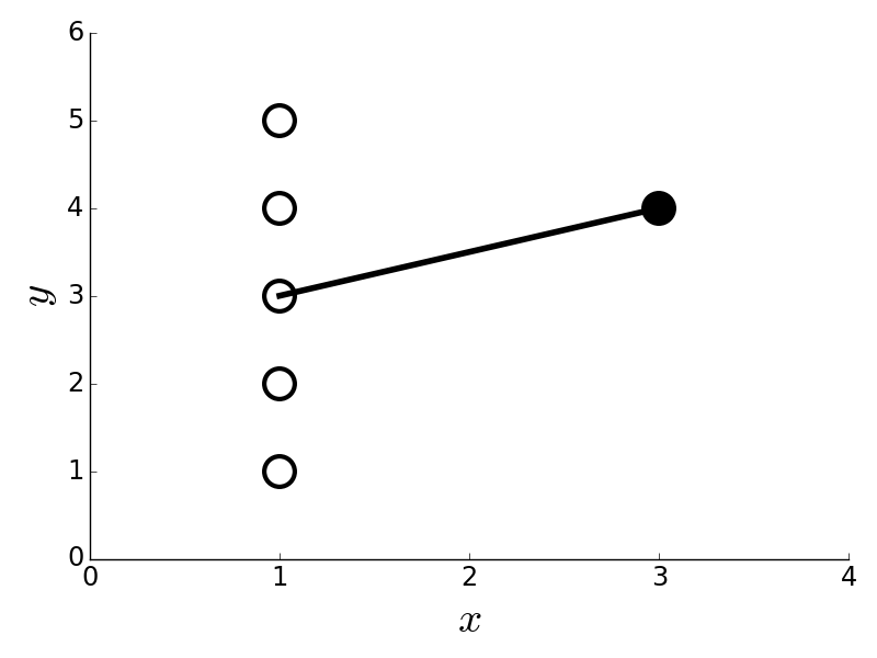
# The point on the right has # outsized influence in this data because it is the only one used to determine the # slope of the fitted line.
# #
#
#
#
# The point on the right in
# [Figure](#fig:Regression_005) is the only one that
# contributes to the
# calculation of the slope for the fitted line. Thus, it
# is very influential in
# this sense. Cook's distance is a good way to get at this
# concept numerically.
# To compute this, we have to compute the $j^{th}$
# component of the estimated
# target variable with the $i^{th}$ point deleted. We
# call this $\hat{y}_{j(i)}$.
# Then, we compute the following,
#
# $$
# D_i =\frac{\sum_j (\hat{y}_j- \hat{y}_{j(i)})^2}{p/n \sum_j (\hat{y}_j-
# y_j)^2}
# $$
#
# where, as before, $p$ is the number of estimated terms
# (e.g., $p=2$ in the
# bivariate case). This calculation emphasizes the
# effect of the outlier by
# predicting the target variable with and
# without each point. In the case of
# [Figure](#fig:Regression_005),
# losing any of the points on the left cannot
# change the estimated
# target variable much, but losing the single point on the
# right surely
# does. The point on the right does not seem to be an outlier (it
# *is*
# on the fitted line), but this is because it is influential enough to
# rotate
# the line to align with it. Cook's distance helps capture this
# effect by leaving
# each sample out and re-fitting the remainder as
# shown in the last equation.
# [Figure](#fig:Regression_006) shows the
# calculated Cook's distance for the data
# in [Figure](#fig:Regression_005), showing that the data point on the right
# (sample index `5`) has outsized influence on the fitted line. As a
# rule of
# thumb, Cook's distance values that are larger than one are
# suspect.
#
#
#
#
#
#
#
#
#
#
# The point on the right in
# [Figure](#fig:Regression_005) is the only one that
# contributes to the
# calculation of the slope for the fitted line. Thus, it
# is very influential in
# this sense. Cook's distance is a good way to get at this
# concept numerically.
# To compute this, we have to compute the $j^{th}$
# component of the estimated
# target variable with the $i^{th}$ point deleted. We
# call this $\hat{y}_{j(i)}$.
# Then, we compute the following,
#
# $$
# D_i =\frac{\sum_j (\hat{y}_j- \hat{y}_{j(i)})^2}{p/n \sum_j (\hat{y}_j-
# y_j)^2}
# $$
#
# where, as before, $p$ is the number of estimated terms
# (e.g., $p=2$ in the
# bivariate case). This calculation emphasizes the
# effect of the outlier by
# predicting the target variable with and
# without each point. In the case of
# [Figure](#fig:Regression_005),
# losing any of the points on the left cannot
# change the estimated
# target variable much, but losing the single point on the
# right surely
# does. The point on the right does not seem to be an outlier (it
# *is*
# on the fitted line), but this is because it is influential enough to
# rotate
# the line to align with it. Cook's distance helps capture this
# effect by leaving
# each sample out and re-fitting the remainder as
# shown in the last equation.
# [Figure](#fig:Regression_006) shows the
# calculated Cook's distance for the data
# in [Figure](#fig:Regression_005), showing that the data point on the right
# (sample index `5`) has outsized influence on the fitted line. As a
# rule of
# thumb, Cook's distance values that are larger than one are
# suspect.
#
#
#
#
#
# The calculated Cook's distance for the data # in [Figure](#fig:Regression_005).
# #
#
#
#
# As another
# illustration of influence, consider [Figure](#fig:Regression_007) which shows
# some data that nicely line up, but
# with one outlier (filled black circle) in the
# upper panel. The lower
# panel shows so-computed Cook's distance for this data
# and emphasizes
# the presence of the outlier. Because the calculation involves
# leaving
# a single sample out and re-calculating the rest, it can be a
# time-
# consuming operation suitable to relatively small data sets. There
# is always the
# temptation to downplay the importance of outliers
# because they conflict with a
# favored model, but outliers must be
# carefully examined to understand why the
# model is unable to capture
# them. It could be something as simple as faulty data
# collection, or it
# could be an indication of deeper issues that have been
# overlooked. The
# following code shows how Cook's distance was compute for
# [Figure](#fig:Regression_006) and [Figure](#fig:Regression_007).
# In[9]:
fit = lambda i,x,y: np.polyval(np.polyfit(x,y,1),i)
omit = lambda i,x: ([k for j,k in enumerate(x) if j !=i])
def cook_d(k):
num = sum((fit(j,omit(k,x),omit(k,y))-fit(j,x,y))**2 for j in x)
den = sum((y-np.polyval(np.polyfit(x,y,1),x))**2/len(x)*2)
return num/den
# **Programming Tip.**
#
# The function `omit` sweeps through the data and excludes
# the $i^{th}$ data element. The embedded `enumerate` function
# associates every
# element in the iterable with its corresponding
# index.
#
#
#
#
#
#
#
#
#
#
#
#
# As another
# illustration of influence, consider [Figure](#fig:Regression_007) which shows
# some data that nicely line up, but
# with one outlier (filled black circle) in the
# upper panel. The lower
# panel shows so-computed Cook's distance for this data
# and emphasizes
# the presence of the outlier. Because the calculation involves
# leaving
# a single sample out and re-calculating the rest, it can be a
# time-
# consuming operation suitable to relatively small data sets. There
# is always the
# temptation to downplay the importance of outliers
# because they conflict with a
# favored model, but outliers must be
# carefully examined to understand why the
# model is unable to capture
# them. It could be something as simple as faulty data
# collection, or it
# could be an indication of deeper issues that have been
# overlooked. The
# following code shows how Cook's distance was compute for
# [Figure](#fig:Regression_006) and [Figure](#fig:Regression_007).
# In[9]:
fit = lambda i,x,y: np.polyval(np.polyfit(x,y,1),i)
omit = lambda i,x: ([k for j,k in enumerate(x) if j !=i])
def cook_d(k):
num = sum((fit(j,omit(k,x),omit(k,y))-fit(j,x,y))**2 for j in x)
den = sum((y-np.polyval(np.polyfit(x,y,1),x))**2/len(x)*2)
return num/den
# **Programming Tip.**
#
# The function `omit` sweeps through the data and excludes
# the $i^{th}$ data element. The embedded `enumerate` function
# associates every
# element in the iterable with its corresponding
# index.
#
#
#
#
#
#
#
# The upper panel shows data that fit on a line # and an outlier point (filled black circle). The lower panel shows the calculated # Cook's distance for the data in upper panel and shows that the tenth point # (i.e., the outlier) has disproportionate influence.
# #
#
#
#