Example decision tree. The Gini coefficient in each branch measures the purity of the partition in each node. The samples item in the box shows the number of items in the corresponding node in the decision tree.
 #
#
# $$
# \texttt{Gini}_m = \sum_k p_{m,k}(1-p_{m,k})
# $$
# where
# $$
# p_{m,k} = \frac{1}{N_m} \sum_{x_i\in R_m} I(y_i=k)
# $$
# which is the proportion of observations labeled $k$ in the $m^{th}$
# node and $I(\cdot)$ is the usual indicator function. Note that the maximum value of
# the Gini coefficient is $\max{\texttt{Gini}_{m}}=1-1/m$. For our simple
# example, half of the sixteen samples are in category `0` and the other half are
# in the `1` category. Using the notation above, the top box corresponds to the
# $0^{th}$ node, so $p_{0,0} =1/2 = p_{0,1}$. Then, $\texttt{Gini}_0=0.5$. The
# next layer of nodes in [Figure](#fig:example_tree_001) is determined by
# whether or not the second dimension of the $\mathbf{x}$ data is greater than
# `1.5`. The Gini coefficients for each of these child nodes is zero because
# after the prior split, each subsequent category is pure. The `value` list in
# each of the nodes shows the distribution of elements in each category at each
# node.
#
# To make this example more interesting, we can contaminate the data slightly,
# In[30]:
M[1,0]=1 # put in different class
print(M) # now contaminated
# Now we have a `1` entry in the previously
# pure first column's second row. Let's re-do
# the analysis as in the following,
# In[31]:
i,j = np.where(M==0)
x=np.vstack([i,j]).T
y = j.reshape(-1,1)*0
i,j = np.where(M==1)
x=np.vstack([np.vstack([i,j]).T,x])
y = np.vstack([j.reshape(-1,1)*0+1,y])
clf.fit(x,y)
# The result is shown
# in [Figure](#fig:example_tree_002). Note the tree has grown
# significantly due to this one change! The $0^{th}$ node has the
# following parameters, $p_{0,0} =7/16$ and $p_{0,1}=9/16$. This makes
# the Gini coefficient for the $0^{th}$ node equal to
# $\frac{7}{16}\left(1-\frac{7}{16}\right)+\frac{9}{16}(1-\frac{9}{16})
# = 0.492$. As before, the root node splits on $X[1] \leq 1.5$. Let's
# see if we can reconstruct the succeeding layer of nodes manually, as
# in the following,
# In[32]:
y[x[:,1]>1.5] # first node on the right
# This obviously has a zero Gini coefficient. Likewise, the node on the
# left contains the following,
# In[33]:
y[x[:,1]<=1.5] # first node on the left
# The Gini coefficient in this case is computed as
# `(1/8)*(1-1/8)+(7/8)*(1-7/8)=0.21875`. This node splits based on `X[1]<0.5`.
# The child node to the right derives from the following equivalent logic,
# In[34]:
np.logical_and(x[:,1]<=1.5,x[:,1]>0.5)
# with corresponding classes,
# In[35]:
y[np.logical_and(x[:,1]<=1.5,x[:,1]>0.5)]
# **Programming Tip.**
#
# The `logical_and` in Numpy provides element-wise logical conjuction. It is not
# possible to accomplish this with something like `0.5< x[:,1] <=1.5` because
# of the way Python parses this syntax.
#
#
#
#
#
#
#
#
#
#
# $$
# \texttt{Gini}_m = \sum_k p_{m,k}(1-p_{m,k})
# $$
# where
# $$
# p_{m,k} = \frac{1}{N_m} \sum_{x_i\in R_m} I(y_i=k)
# $$
# which is the proportion of observations labeled $k$ in the $m^{th}$
# node and $I(\cdot)$ is the usual indicator function. Note that the maximum value of
# the Gini coefficient is $\max{\texttt{Gini}_{m}}=1-1/m$. For our simple
# example, half of the sixteen samples are in category `0` and the other half are
# in the `1` category. Using the notation above, the top box corresponds to the
# $0^{th}$ node, so $p_{0,0} =1/2 = p_{0,1}$. Then, $\texttt{Gini}_0=0.5$. The
# next layer of nodes in [Figure](#fig:example_tree_001) is determined by
# whether or not the second dimension of the $\mathbf{x}$ data is greater than
# `1.5`. The Gini coefficients for each of these child nodes is zero because
# after the prior split, each subsequent category is pure. The `value` list in
# each of the nodes shows the distribution of elements in each category at each
# node.
#
# To make this example more interesting, we can contaminate the data slightly,
# In[30]:
M[1,0]=1 # put in different class
print(M) # now contaminated
# Now we have a `1` entry in the previously
# pure first column's second row. Let's re-do
# the analysis as in the following,
# In[31]:
i,j = np.where(M==0)
x=np.vstack([i,j]).T
y = j.reshape(-1,1)*0
i,j = np.where(M==1)
x=np.vstack([np.vstack([i,j]).T,x])
y = np.vstack([j.reshape(-1,1)*0+1,y])
clf.fit(x,y)
# The result is shown
# in [Figure](#fig:example_tree_002). Note the tree has grown
# significantly due to this one change! The $0^{th}$ node has the
# following parameters, $p_{0,0} =7/16$ and $p_{0,1}=9/16$. This makes
# the Gini coefficient for the $0^{th}$ node equal to
# $\frac{7}{16}\left(1-\frac{7}{16}\right)+\frac{9}{16}(1-\frac{9}{16})
# = 0.492$. As before, the root node splits on $X[1] \leq 1.5$. Let's
# see if we can reconstruct the succeeding layer of nodes manually, as
# in the following,
# In[32]:
y[x[:,1]>1.5] # first node on the right
# This obviously has a zero Gini coefficient. Likewise, the node on the
# left contains the following,
# In[33]:
y[x[:,1]<=1.5] # first node on the left
# The Gini coefficient in this case is computed as
# `(1/8)*(1-1/8)+(7/8)*(1-7/8)=0.21875`. This node splits based on `X[1]<0.5`.
# The child node to the right derives from the following equivalent logic,
# In[34]:
np.logical_and(x[:,1]<=1.5,x[:,1]>0.5)
# with corresponding classes,
# In[35]:
y[np.logical_and(x[:,1]<=1.5,x[:,1]>0.5)]
# **Programming Tip.**
#
# The `logical_and` in Numpy provides element-wise logical conjuction. It is not
# possible to accomplish this with something like `0.5< x[:,1] <=1.5` because
# of the way Python parses this syntax.
#
#
#
#
#
#
#
# Decision tree for contaminated data. Note that just one change in the training data caused the tree to grow five times as large as before!
# #
#
#
#
# Notice that for this example as well as for the previous one, the decision tree
# was exactly able memorize (overfit) the data with perfect accuracy. From our
# discussion of machine learning theory, this is an indication potential problems
# in generalization.
#
#
# The key step in building the decision tree is to come up with the
# initial split. There are the number of algorithms that can build
# decision trees based on different criteria, but the general idea is to
# control the information *entropy* as the tree is developed. In
# practical terms, this means that the algorithms attempt to build trees
# that are not excessively deep. It is well-established that this is a
# very hard problem to solve completely and there are many approaches to
# it. This is because the algorithms must make global decisions at each
# node of the tree using the local data available up to that point.
# In[36]:
_=clf.fit(x,y)
fig,axs=subplots(2,2,sharex=True,sharey=True)
ax=axs[0,0]
ax.set_aspect(1)
_=ax.axis((-1,4,-1,4))
ax.invert_yaxis()
# same background all on axes
for ax in axs.flat:
_=ax.plot(ma.masked_array(x[:,1],y==1),ma.masked_array(x[:,0],y==1),'ow',mec='k')
_=ax.plot(ma.masked_array(x[:,1],y==0),ma.masked_array(x[:,0],y==0),'o',color='gray')
lines={'h':[],'v':[]}
nc=0
for i,j,ax in zip(clf.tree_.feature,clf.tree_.threshold,axs.flat):
_=ax.set_title('node %d'%(nc))
nc+=1
if i==0: _=lines['h'].append(j)
elif i==1: _=lines['v'].append(j)
for l in lines['v']: _=ax.vlines(l,-1,4,lw=3)
for l in lines['h']: _=ax.hlines(l,-1,4,lw=3)
fig.savefig('fig-machine_learning/example_tree_003.png')
#
#
#
#
#
#
#
#
#
# Notice that for this example as well as for the previous one, the decision tree
# was exactly able memorize (overfit) the data with perfect accuracy. From our
# discussion of machine learning theory, this is an indication potential problems
# in generalization.
#
#
# The key step in building the decision tree is to come up with the
# initial split. There are the number of algorithms that can build
# decision trees based on different criteria, but the general idea is to
# control the information *entropy* as the tree is developed. In
# practical terms, this means that the algorithms attempt to build trees
# that are not excessively deep. It is well-established that this is a
# very hard problem to solve completely and there are many approaches to
# it. This is because the algorithms must make global decisions at each
# node of the tree using the local data available up to that point.
# In[36]:
_=clf.fit(x,y)
fig,axs=subplots(2,2,sharex=True,sharey=True)
ax=axs[0,0]
ax.set_aspect(1)
_=ax.axis((-1,4,-1,4))
ax.invert_yaxis()
# same background all on axes
for ax in axs.flat:
_=ax.plot(ma.masked_array(x[:,1],y==1),ma.masked_array(x[:,0],y==1),'ow',mec='k')
_=ax.plot(ma.masked_array(x[:,1],y==0),ma.masked_array(x[:,0],y==0),'o',color='gray')
lines={'h':[],'v':[]}
nc=0
for i,j,ax in zip(clf.tree_.feature,clf.tree_.threshold,axs.flat):
_=ax.set_title('node %d'%(nc))
nc+=1
if i==0: _=lines['h'].append(j)
elif i==1: _=lines['v'].append(j)
for l in lines['v']: _=ax.vlines(l,-1,4,lw=3)
for l in lines['h']: _=ax.hlines(l,-1,4,lw=3)
fig.savefig('fig-machine_learning/example_tree_003.png')
#
#
#
#
# The decision tree divides the training set into regions by splitting successively along each dimension until each region is as pure as possible.
# #
#
#
#
# For this example, the decision tree partitions the $\mathcal{X}$ space into
# different regions corresponding to different $\mathcal{Y}$ labels as shown in
# [Figure](#fig:example_tree_003). The root node at the top of [Figure](#fig:example_tree_002) splits the input data based on $X[1] \leq 1.5$. This
# corresponds to the top left panel in [Figure](#fig:example_tree_003) (i.e.,
# `node 0`) where the vertical line divides the training data shown into two
# regions, corresponding to the two subsequent child nodes. The next split
# happens with $X[1] \leq 0.5$ as shown in the next panel of [Figure](#fig:example_tree_003) titled `node 1`. This continues until the last panel
# on the lower right, where the contaminated element we injected has been
# isolated into its own sub-region. Thus, the last panel is a representation of
# [Figure](#fig:example_tree_002), where the horizontal/vertical lines
# correspond to successive splits in the decision tree.
# In[37]:
i,j = np.indices((5,5))
x=np.vstack([i.flatten(),j.flatten()]).T
y=(x[:,0]>=x[:,1]).astype(int).reshape((-1,1))
_=clf.fit(x,y)
fig,ax=subplots()
_=ax.axis((-1,5,-1,5))
ax.set_aspect(1)
ax.invert_yaxis()
_=ax.plot(ma.masked_array(x[:,1],y==1),ma.masked_array(x[:,0],y==1),'ow',mec='k',ms=15)
_=ax.plot(ma.masked_array(x[:,1],y==0),ma.masked_array(x[:,0],y==0),'o',color='gray',ms=15)
for i,j in zip(clf.tree_.feature,clf.tree_.threshold):
if i==1:
_=ax.hlines(j,-1,6,lw=3.)
else:
_=ax.vlines(j,-1,6,lw=3.)
fig.savefig('fig-machine_learning/example_tree_004.png')
#
#
#
#
#
#
#
#
#
# For this example, the decision tree partitions the $\mathcal{X}$ space into
# different regions corresponding to different $\mathcal{Y}$ labels as shown in
# [Figure](#fig:example_tree_003). The root node at the top of [Figure](#fig:example_tree_002) splits the input data based on $X[1] \leq 1.5$. This
# corresponds to the top left panel in [Figure](#fig:example_tree_003) (i.e.,
# `node 0`) where the vertical line divides the training data shown into two
# regions, corresponding to the two subsequent child nodes. The next split
# happens with $X[1] \leq 0.5$ as shown in the next panel of [Figure](#fig:example_tree_003) titled `node 1`. This continues until the last panel
# on the lower right, where the contaminated element we injected has been
# isolated into its own sub-region. Thus, the last panel is a representation of
# [Figure](#fig:example_tree_002), where the horizontal/vertical lines
# correspond to successive splits in the decision tree.
# In[37]:
i,j = np.indices((5,5))
x=np.vstack([i.flatten(),j.flatten()]).T
y=(x[:,0]>=x[:,1]).astype(int).reshape((-1,1))
_=clf.fit(x,y)
fig,ax=subplots()
_=ax.axis((-1,5,-1,5))
ax.set_aspect(1)
ax.invert_yaxis()
_=ax.plot(ma.masked_array(x[:,1],y==1),ma.masked_array(x[:,0],y==1),'ow',mec='k',ms=15)
_=ax.plot(ma.masked_array(x[:,1],y==0),ma.masked_array(x[:,0],y==0),'o',color='gray',ms=15)
for i,j in zip(clf.tree_.feature,clf.tree_.threshold):
if i==1:
_=ax.hlines(j,-1,6,lw=3.)
else:
_=ax.vlines(j,-1,6,lw=3.)
fig.savefig('fig-machine_learning/example_tree_004.png')
#
#
#
#
# The decision tree fitted to this triangular matrix is very complex, as shown by the number of horizontal and vertical partitions. Thus, even though the pattern in the training data is visually clear, the decision tree cannot automatically uncover it.
# #
#
#
#
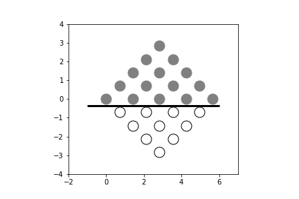
# [Figure](#fig:example_tree_004) shows another example, but now using a simple
# triangular matrix. As shown by the number of vertical and horizontal
# partitioning lines, the decision tree that corresponds to this figure is tall
# and complex. Notice that if we apply a simple rotational transform to the
# training data, we can obtain [Figure](#fig:example_tree_005), which requires a
# trivial decision tree to fit. Thus, there may be transformations of the
# training data that simplify the decision tree, but these are very difficult to
# derive in general. Nonetheless, this highlights a key weakness of decision
# trees wherein they may be easy to understand, to train, and to deploy, but may
# be completely blind to such time-saving and complexity-saving transformations.
# Indeed, in higher dimensions, it may be impossible to even visualize the
# potential of such latent transformations. Thus, the advantages of decision
# trees can be easily outmatched by other methods that we will study later that
# *do* have the ability to uncover useful transformations, but which will
# necessarily be harder to train. Another disadvantage is that because of how
# decision trees are built, even a single misplaced data point can cause the tree
# to grow very differently. This is a symptom of high variance.
#
# In all of our examples, the decision tree was able to
# memorize the training data exactly, as we discussed earlier,
# this is a sign of potentially high generalization errors. There
# are pruning algorithms that strategically remove some of the
# deepest nodes. but these are not yet fully implemented in
# Scikit-learn, as of this writing. Alternatively, restricting
# the maximum depth of the decision tree can have a similar
# effect. The `DecisionTreeClassifier` and
# `DecisionTreeRegressor` in Scikit-learn both have keyword
# arguments that specify maximum depth.
#
# ## Random Forests
#
# It is possible to combine a set of decision trees into a larger
# composite tree that has better performance than its individual
# components by using ensemble learning. This is implemented in
# Scikit-learn as `RandomForestClassifier`. The composite tree helps
# mitigate the primary weakness of decision trees --- high variance.
# Random forest classifiers help by averaging out the predictions of
# many constituent trees to minimize this variance by randomly selecting
# subsets of the training set to train the embedded trees. On the
# other hand, this randomization can increase bias because there may be
# a subset of the training set that yields an excellent decision tree,
# but the averaging effect over randomized training samples washes this
# out in the same averaging that reduces the variance. This is a key
# trade-off. The following code implements a simple random forest
# classifer from our last example.
# In[38]:
from numpy import sin, cos, pi
rotation_matrix=np.matrix([[cos(pi/4),-sin(pi/4)],
[sin(pi/4),cos(pi/4)]])
xr=(rotation_matrix*(x.T)).T
xr=np.array(xr)
fig,ax=subplots()
ax.set_aspect(1)
_=ax.axis(xmin=-2,xmax=7,ymin=-4,ymax=4)
_=ax.plot(ma.masked_array(xr[:,1],y==1),ma.masked_array(xr[:,0],y==1),'ow',mec='k',ms=15)
_=ax.plot(ma.masked_array(xr[:,1],y==0),ma.masked_array(xr[:,0],y==0),'o',color='gray',ms=15)
_=clf.fit(xr,y)
for i,j in zip(clf.tree_.feature,clf.tree_.threshold):
if i==1:
_=ax.vlines(j,-1,6,lw=3.)
elif i==0:
_=ax.hlines(j,-1,6,lw=3.)
fig.savefig('fig-machine_learning/example_tree_005.png')
#
#
#
#
#
#
#
#
#
# [Figure](#fig:example_tree_004) shows another example, but now using a simple
# triangular matrix. As shown by the number of vertical and horizontal
# partitioning lines, the decision tree that corresponds to this figure is tall
# and complex. Notice that if we apply a simple rotational transform to the
# training data, we can obtain [Figure](#fig:example_tree_005), which requires a
# trivial decision tree to fit. Thus, there may be transformations of the
# training data that simplify the decision tree, but these are very difficult to
# derive in general. Nonetheless, this highlights a key weakness of decision
# trees wherein they may be easy to understand, to train, and to deploy, but may
# be completely blind to such time-saving and complexity-saving transformations.
# Indeed, in higher dimensions, it may be impossible to even visualize the
# potential of such latent transformations. Thus, the advantages of decision
# trees can be easily outmatched by other methods that we will study later that
# *do* have the ability to uncover useful transformations, but which will
# necessarily be harder to train. Another disadvantage is that because of how
# decision trees are built, even a single misplaced data point can cause the tree
# to grow very differently. This is a symptom of high variance.
#
# In all of our examples, the decision tree was able to
# memorize the training data exactly, as we discussed earlier,
# this is a sign of potentially high generalization errors. There
# are pruning algorithms that strategically remove some of the
# deepest nodes. but these are not yet fully implemented in
# Scikit-learn, as of this writing. Alternatively, restricting
# the maximum depth of the decision tree can have a similar
# effect. The `DecisionTreeClassifier` and
# `DecisionTreeRegressor` in Scikit-learn both have keyword
# arguments that specify maximum depth.
#
# ## Random Forests
#
# It is possible to combine a set of decision trees into a larger
# composite tree that has better performance than its individual
# components by using ensemble learning. This is implemented in
# Scikit-learn as `RandomForestClassifier`. The composite tree helps
# mitigate the primary weakness of decision trees --- high variance.
# Random forest classifiers help by averaging out the predictions of
# many constituent trees to minimize this variance by randomly selecting
# subsets of the training set to train the embedded trees. On the
# other hand, this randomization can increase bias because there may be
# a subset of the training set that yields an excellent decision tree,
# but the averaging effect over randomized training samples washes this
# out in the same averaging that reduces the variance. This is a key
# trade-off. The following code implements a simple random forest
# classifer from our last example.
# In[38]:
from numpy import sin, cos, pi
rotation_matrix=np.matrix([[cos(pi/4),-sin(pi/4)],
[sin(pi/4),cos(pi/4)]])
xr=(rotation_matrix*(x.T)).T
xr=np.array(xr)
fig,ax=subplots()
ax.set_aspect(1)
_=ax.axis(xmin=-2,xmax=7,ymin=-4,ymax=4)
_=ax.plot(ma.masked_array(xr[:,1],y==1),ma.masked_array(xr[:,0],y==1),'ow',mec='k',ms=15)
_=ax.plot(ma.masked_array(xr[:,1],y==0),ma.masked_array(xr[:,0],y==0),'o',color='gray',ms=15)
_=clf.fit(xr,y)
for i,j in zip(clf.tree_.feature,clf.tree_.threshold):
if i==1:
_=ax.vlines(j,-1,6,lw=3.)
elif i==0:
_=ax.hlines(j,-1,6,lw=3.)
fig.savefig('fig-machine_learning/example_tree_005.png')
#
#
#
#
# Using a simple rotation on the training data in [Figure](#fig:example_tree_004), the decision tree can now easily fit the training data with a single partition.
# #
#
# In[39]:
from sklearn.ensemble import RandomForestClassifier
from sklearn.model_selection import train_test_split, cross_val_score
X_train,X_test,y_train,y_test=train_test_split(x,y,random_state=1)
clf = tree.DecisionTreeClassifier(max_depth=2)
_=clf.fit(X_train,y_train)
rfc = RandomForestClassifier(n_estimators=4,max_depth=2)
_=rfc.fit(X_train,y_train.flat)
# In[40]:
from sklearn.ensemble import RandomForestClassifier
rfc = RandomForestClassifier(n_estimators=4,max_depth=2)
rfc.fit(X_train,y_train.flat)
# In[41]:
def draw_board(x,y,clf,ax=None):
if ax is None: fig,ax=subplots()
xm,ymn=x.min(0).T
ax.axis(xmin=xm-1,ymin=ymn-1)
xx,ymx=x.max(0).T
_=ax.axis(xmax=xx+1,ymax=ymx+1)
_=ax.set_aspect(1)
_=ax.invert_yaxis()
_=ax.plot(ma.masked_array(x[:,1],y==1),ma.masked_array(x[:,0],y==1),'ow',mec='k')
_=ax.plot(ma.masked_array(x[:,1],y==0),ma.masked_array(x[:,0],y==0),'o',color='gray')
for i,j in zip(clf.tree_.feature,clf.tree_.threshold):
if i==1:
_=ax.vlines(j,-1,6,lw=3.)
elif i==0:
_=ax.hlines(j,-1,6,lw=3.)
return ax
# In[42]:
fig,axs = subplots(2,2)
# draw constituent decision trees
for est,ax in zip(rfc.estimators_,axs.flat):
_=draw_board(X_train,y_train,est,ax=ax)
fig.savefig('fig-machine_learning/example_tree_006.png')
# Note that we have constrained the maximum depth `max_depth=2` to help
# with generalization. To keep things simple we have only set up a forest with
# four individual classifers [^seedNote]. [Figure](#fig:example_tree_006) shows
# the individual classifers in the forest that have been trained above. Even
# though all the constituent decision trees share the same training data, the
# random forest algorithm randomly picks feature subsets (with replacement) upon
# which to train individual trees. This helps avoid the tendency of decision
# trees to become too deep and lopsided, which hurts both performance and
# generalization. At the prediction step, the individual outputs of each of the
# constituent decision trees are put to a majority vote for the final
# classification. To estimate generalization errors without using
# cross-validation, the training elements *not* used for a particular constituent
# tree can be used to test that tree and form a collaborative estimate of
# generalization errors. This is called the *out-of-bag* estimate.
#
# [^seedNote]: We have also set the random seed to a fixed value
# to make the figures reproducible in the Jupyter Notebook corresponding to
# this section.
#
#
#
#
#
#
#
#
# In[39]:
from sklearn.ensemble import RandomForestClassifier
from sklearn.model_selection import train_test_split, cross_val_score
X_train,X_test,y_train,y_test=train_test_split(x,y,random_state=1)
clf = tree.DecisionTreeClassifier(max_depth=2)
_=clf.fit(X_train,y_train)
rfc = RandomForestClassifier(n_estimators=4,max_depth=2)
_=rfc.fit(X_train,y_train.flat)
# In[40]:
from sklearn.ensemble import RandomForestClassifier
rfc = RandomForestClassifier(n_estimators=4,max_depth=2)
rfc.fit(X_train,y_train.flat)
# In[41]:
def draw_board(x,y,clf,ax=None):
if ax is None: fig,ax=subplots()
xm,ymn=x.min(0).T
ax.axis(xmin=xm-1,ymin=ymn-1)
xx,ymx=x.max(0).T
_=ax.axis(xmax=xx+1,ymax=ymx+1)
_=ax.set_aspect(1)
_=ax.invert_yaxis()
_=ax.plot(ma.masked_array(x[:,1],y==1),ma.masked_array(x[:,0],y==1),'ow',mec='k')
_=ax.plot(ma.masked_array(x[:,1],y==0),ma.masked_array(x[:,0],y==0),'o',color='gray')
for i,j in zip(clf.tree_.feature,clf.tree_.threshold):
if i==1:
_=ax.vlines(j,-1,6,lw=3.)
elif i==0:
_=ax.hlines(j,-1,6,lw=3.)
return ax
# In[42]:
fig,axs = subplots(2,2)
# draw constituent decision trees
for est,ax in zip(rfc.estimators_,axs.flat):
_=draw_board(X_train,y_train,est,ax=ax)
fig.savefig('fig-machine_learning/example_tree_006.png')
# Note that we have constrained the maximum depth `max_depth=2` to help
# with generalization. To keep things simple we have only set up a forest with
# four individual classifers [^seedNote]. [Figure](#fig:example_tree_006) shows
# the individual classifers in the forest that have been trained above. Even
# though all the constituent decision trees share the same training data, the
# random forest algorithm randomly picks feature subsets (with replacement) upon
# which to train individual trees. This helps avoid the tendency of decision
# trees to become too deep and lopsided, which hurts both performance and
# generalization. At the prediction step, the individual outputs of each of the
# constituent decision trees are put to a majority vote for the final
# classification. To estimate generalization errors without using
# cross-validation, the training elements *not* used for a particular constituent
# tree can be used to test that tree and form a collaborative estimate of
# generalization errors. This is called the *out-of-bag* estimate.
#
# [^seedNote]: We have also set the random seed to a fixed value
# to make the figures reproducible in the Jupyter Notebook corresponding to
# this section.
#
#
#
#
#
# The constituent decision trees of the random forest and how they partitioned the training set are shown in these four panels. The random forest classifier uses the individual outputs of each of the constituent trees to produce a collaborative final estimate.
# #
#
#
#
# The main advantage of random forest classifiers is that they require very
# little tuning and provide a way to trade-off bias and variance via averaging
# and randomization. Furthermore, they are fast and easy to train in parallel
# (see the `n_jobs` keyword argument) and fast to predict. On the downside, they
# are less interpretable than simple decision trees. There are many other
# powerful tree methods in Scikit-learn like `ExtraTrees` and Gradient Boosted
# Regression Trees `GradientBoostingRegressor` which are discussed in the online
# documentation.
#
#
#
#
#
#
#
#
# ## Boosting Trees
#
# To understand additive modeling using trees, recall the
# Gram-Schmidt orthogonalization procedure for vectors. The
# purpose of this orthogonalization procedure is to create an
# orthogonal set of vectors starting with a given vector
# $\mathbf{u}_1$. We have already discussed the projection
# operator in the section [ch:prob:sec:projection](#ch:prob:sec:projection). The
# Gram-Schmidt orthogonalization procedure starts with a
# vector $\mathbf{v}_1$, which we define as the following:
# $$
# \mathbf{u}_1 = \mathbf{v}_1
# $$
# with the corresponding projection operator $proj_{\mathbf{u}_1}$. The
# next step in the procedure is to remove the residual of $\mathbf{u}_1$
# from $\mathbf{v}_2$, as in the following:
# $$
# \mathbf{u}_2 = \mathbf{v}_2 - proj_{\mathbf{u}_1}(\mathbf{v}_2)
# $$
# This procedure continues for $\mathbf{v}_3$ as in the following:
# $$
# \mathbf{u}_3 = \mathbf{v}_3 - proj_{\mathbf{u}_1}(\mathbf{v}_3) - proj_{\mathbf{u}_2}(\mathbf{v}_3)
# $$
# and so on. The important aspect of this procedure is that new
# incoming vectors (i.e., $\mathbf{v}_k$) are stripped of any pre-existing
# components already present in the set of $\lbrace\mathbf{u}_1,\mathbf{u}_2,\ldots,\mathbf{u}_M \rbrace$.
#
# Note that this procedure is sequential. That is, the *order*
# of the incoming $\mathbf{v}_i$ matters [^rotation]. Thus,
# any new vector can be expressed using the so-constructed
# $\lbrace\mathbf{u}_1,\mathbf{u}_2,\ldots,\mathbf{u}_M
# \rbrace$ basis set, as in the following:
#
# [^rotation]: At least up to a rotation of the resulting
# orthonormal basis.
# $$
# \mathbf{x} = \sum \alpha_i \mathbf{u}_i
# $$
# The idea behind additive trees is to reproduce this procedure for
# trees instead of vectors. There are many natural topological and algebraic
# properties that we lack for the general problem, however. For example, we already
# have well established methods for measuring distances between vectors for
# the Gram-Schmidt procedure outlined above (namely, the $L_2$
# distance), which we lack here. Thus, we need the concept of *loss function*,
# which is a way of measuring how well the process is working out at each
# sequential step. This loss function is parameterized by the training data and
# by the classification function under consideration: $ L_{\mathbf{y}}(f(x)) $.
# For example, if we want a classifier ($f$) that selects the label $y_i$
# based upon the input data $\mathbf{x}_i$ ($f :\mathbf{x}_i \rightarrow y_i)$,
# then the squared error loss function would be the following:
# $$
# L_{\mathbf{y}}(f(x)) = \sum_i (y_i - f(x_i))^2
# $$
# We represent the classifier in terms of a set of basis trees:
# $$
# f(x) = \sum_k \alpha_k u_{\mathbf{x}}(\theta_k)
# $$
# The general algorithm for forward stagewise additive modeling is
# the following:
#
# * Initialize $f(x)=0$
#
# * For $m=1$ to $m=M$, compute the following:
# $$
# (\beta_m,\gamma_m) = \argmin_{\beta,\gamma} \sum_i L(y_i,f_{m-1}(x_i)+\beta b(x_i;\gamma))
# $$
# * Set $f_m(x) = f_{m-1}(x) +\beta_m b(x;\gamma_m) $
#
# The key point is that the residuals from the prior step are used to fit the
# basis function for the subsequent iteration. That is, the following
# equation is being sequentially approximated.
# $$
# f_m(x) - f_{m-1}(x) =\beta_m b(x_i;\gamma_m)
# $$
# Let's see how this works for decision trees and the exponential loss
# function.
# $$
# L(x,f(x)) = \exp(-y f(x))
# $$
# Recall that for the classification problem, $y\in \lbrace -1,1 \rbrace$. For
# AdaBoost, the basis functions are the individual classifiers, $G_m(x)\mapsto \lbrace -1,1 \rbrace$
# The key step in the algorithm is the minimization step for
# the objective function
# $$
# J(\beta,G) = \sum_i \exp(y_i(f_{m-1}(x_i)+\beta G(x_i)))
# $$
# $$
# (\beta_m,G_m) = \argmin_{\beta,G} \sum_i \exp(y_i(f_{m-1}(x_i)+\beta G(x_i)))
# $$
# Now, because of the exponential, we can factor out the following:
# $$
# w_i^{(m)} = \exp(y_i f_{m-1}(x_i))
# $$
# as a weight on each data element and re-write the objective function as the following:
# $$
# J(\beta,G) = \sum_i w_i^{(m)} \exp(y_i \beta G(x_i))
# $$
# The important observation here is that $y_i G(x_i)\mapsto 1$ if
# the tree classifies $x_i$ correctly and $y_i G(x_i)\mapsto -1$ otherwise.
# Thus, the above sum has terms like the following:
# $$
# J(\beta,G) = \sum_{y_i\ne G(x_i)} w_i^{(m)} \exp(-\beta) + \sum_{y_i= G(x_i)} w_i^{(m)}\exp(\beta)
# $$
# For $\beta>0$, this means that the best $G(x)$ is
# the one that incorrectly classifies for the largest weights. Thus,
# the minimizer is the following:
# $$
# G_m = \argmin_G \sum_i w_i^{(m)} I(y_i \ne G(x_i))
# $$
# where $I$ is the indicator function (i.e.,
# $I(\texttt{True})=1,I(\texttt{False})=0$).
#
# For $\beta>0$, we can re-write the objective function
# as the following:
# $$
# J= (\exp(\beta)-\exp(-\beta))\sum_i w_i^{(m)} I(y_i \ne G(x_i)) + \exp(-\beta) \sum_i w_i^{(m)}
# $$
# and substitute $\theta=\exp(-\beta)$ so that
#
#
#
# $$
# \begin{equation}
# \frac{J}{\sum_i w_i^{(m)}} = \left(\frac{1}{\theta} - \theta\right)\epsilon_m+\theta
# \label{eq:bt001} \tag{1}
# \end{equation}
# $$
# where
# $$
# \epsilon_m = \frac{\sum_i w_i^{(m)}I(y_i\ne G(x_i))}{\sum_i w_i^{(m)}}
# $$
# is the error rate of the classifier with $0\le \epsilon_m\le 1$. Now,
# finding $\beta$ is a straight-forward calculus minimization exercise on the
# right side of Equation ([1](#eq:bt001)), which gives the following:
# $$
# \beta_m = \frac{1}{2}\log \frac{1-\epsilon_m}{\epsilon_m}
# $$
# Importantly, $\beta_m$ can become negative if
# $\epsilon_m<\frac{1}{2}$, which would would violate our assumptions on $\beta$.
# This is captured in the requirement that the base learner be better than just
# random guessing, which would correspond to $\epsilon_m>\frac{1}{2}$.
# Practically speaking, this means that boosting cannot fix a base learner that
# is no better than a random guess. Formally speaking, this is known as the
# *empirical weak learning assumption* [[schapire2012boosting]](#schapire2012boosting).
#
# Now we can move to the iterative weight update. Recall that
# $$
# w_i^{(m+1)} = \exp(y_i f_{m}(x_i)) = w_i^{(m)}\exp(y_i \beta_m G_m(x_i))
# $$
# which we can rewrite as the following:
# $$
# w_i^{(m+1)} = w_i^{(m)}\exp(\beta_m)\exp(-2\beta_m I(G_m(x_i)=y_i))
# $$
# This means that the data elements that are incorrectly classified have their
# corresponding weights increased by $\exp(\beta_m)$ and those that are correctly
# classified have their corresponding weights reduced by $\exp(-\beta_m)$.
# The reason for the choice of the exponential loss function comes from the
# following:
# $$
# f^{*}(x) = \argmin_{f(x)} \mathbb{E}_{Y\vert x}(\exp(-Y f(x))) = \frac{1}{2}\log \frac{\mathbb{P}(Y=1\vert x)}{\mathbb{P}(Y=\minus 1\vert x)}
# $$
# This means that boosting is approximating a $f(x)$ that is actually
# half the log-odds of the conditional class probabilities. This can be
# rearranged as the following
# $$
# \mathbb{P}(Y=1\vert x) = \frac{1}{1+\exp(\minus 2f^{*}(x))}
# $$
# The important benefit of this general formulation for boosting, as a sequence
# of additive approximations, is that it opens the door to other choices of loss
# function, especially loss functions that are based on robust statistics that
# can account for errors in the training data (c.f. Hastie).
#
# ### Gradient Boosting
#
# Given a differentiable loss function, the optimization process can be
# formulated using numerical gradients. The fundamental idea is to treat the
# $f(x_i)$ as a scalar parameter to be optimized over. Generally speaking,
# we can think of the following loss function,
# $$
# L(f) = \sum_{i=1}^N L(y_i,f(x_i))
# $$
# as a vectorized quantity
# $$
# \mathbf{f} = \lbrace f(x_1),f(x_2),\ldots, f(x_N) \rbrace
# $$
# so that the optimization is over this vector
# $$
# \hat{\mathbf{f}} = \argmin_{\mathbf{f}} L(\mathbf{f})
# $$
# With this general formulation we can use numerical optimization methods
# to solve for the optimal $\mathbf{f}$ as a sum of component vectors
# as in the following:
# $$
# \mathbf{f}_M = \sum_{m=0}^M \mathbf{h}_m
# $$
# Note that this leaves aside the prior assumption that $f$
# is parameterized as a sum of individual decision trees.
# $$
# g_{i,m} = \left[ \frac{\partial L(y_i,f(x_i))}{\partial f(x_i)} \right]_{f(x_i)=f_{m-1}(x_i)}
# $$
#
#
#
#
#
#
# The main advantage of random forest classifiers is that they require very
# little tuning and provide a way to trade-off bias and variance via averaging
# and randomization. Furthermore, they are fast and easy to train in parallel
# (see the `n_jobs` keyword argument) and fast to predict. On the downside, they
# are less interpretable than simple decision trees. There are many other
# powerful tree methods in Scikit-learn like `ExtraTrees` and Gradient Boosted
# Regression Trees `GradientBoostingRegressor` which are discussed in the online
# documentation.
#
#
#
#
#
#
#
#
# ## Boosting Trees
#
# To understand additive modeling using trees, recall the
# Gram-Schmidt orthogonalization procedure for vectors. The
# purpose of this orthogonalization procedure is to create an
# orthogonal set of vectors starting with a given vector
# $\mathbf{u}_1$. We have already discussed the projection
# operator in the section [ch:prob:sec:projection](#ch:prob:sec:projection). The
# Gram-Schmidt orthogonalization procedure starts with a
# vector $\mathbf{v}_1$, which we define as the following:
# $$
# \mathbf{u}_1 = \mathbf{v}_1
# $$
# with the corresponding projection operator $proj_{\mathbf{u}_1}$. The
# next step in the procedure is to remove the residual of $\mathbf{u}_1$
# from $\mathbf{v}_2$, as in the following:
# $$
# \mathbf{u}_2 = \mathbf{v}_2 - proj_{\mathbf{u}_1}(\mathbf{v}_2)
# $$
# This procedure continues for $\mathbf{v}_3$ as in the following:
# $$
# \mathbf{u}_3 = \mathbf{v}_3 - proj_{\mathbf{u}_1}(\mathbf{v}_3) - proj_{\mathbf{u}_2}(\mathbf{v}_3)
# $$
# and so on. The important aspect of this procedure is that new
# incoming vectors (i.e., $\mathbf{v}_k$) are stripped of any pre-existing
# components already present in the set of $\lbrace\mathbf{u}_1,\mathbf{u}_2,\ldots,\mathbf{u}_M \rbrace$.
#
# Note that this procedure is sequential. That is, the *order*
# of the incoming $\mathbf{v}_i$ matters [^rotation]. Thus,
# any new vector can be expressed using the so-constructed
# $\lbrace\mathbf{u}_1,\mathbf{u}_2,\ldots,\mathbf{u}_M
# \rbrace$ basis set, as in the following:
#
# [^rotation]: At least up to a rotation of the resulting
# orthonormal basis.
# $$
# \mathbf{x} = \sum \alpha_i \mathbf{u}_i
# $$
# The idea behind additive trees is to reproduce this procedure for
# trees instead of vectors. There are many natural topological and algebraic
# properties that we lack for the general problem, however. For example, we already
# have well established methods for measuring distances between vectors for
# the Gram-Schmidt procedure outlined above (namely, the $L_2$
# distance), which we lack here. Thus, we need the concept of *loss function*,
# which is a way of measuring how well the process is working out at each
# sequential step. This loss function is parameterized by the training data and
# by the classification function under consideration: $ L_{\mathbf{y}}(f(x)) $.
# For example, if we want a classifier ($f$) that selects the label $y_i$
# based upon the input data $\mathbf{x}_i$ ($f :\mathbf{x}_i \rightarrow y_i)$,
# then the squared error loss function would be the following:
# $$
# L_{\mathbf{y}}(f(x)) = \sum_i (y_i - f(x_i))^2
# $$
# We represent the classifier in terms of a set of basis trees:
# $$
# f(x) = \sum_k \alpha_k u_{\mathbf{x}}(\theta_k)
# $$
# The general algorithm for forward stagewise additive modeling is
# the following:
#
# * Initialize $f(x)=0$
#
# * For $m=1$ to $m=M$, compute the following:
# $$
# (\beta_m,\gamma_m) = \argmin_{\beta,\gamma} \sum_i L(y_i,f_{m-1}(x_i)+\beta b(x_i;\gamma))
# $$
# * Set $f_m(x) = f_{m-1}(x) +\beta_m b(x;\gamma_m) $
#
# The key point is that the residuals from the prior step are used to fit the
# basis function for the subsequent iteration. That is, the following
# equation is being sequentially approximated.
# $$
# f_m(x) - f_{m-1}(x) =\beta_m b(x_i;\gamma_m)
# $$
# Let's see how this works for decision trees and the exponential loss
# function.
# $$
# L(x,f(x)) = \exp(-y f(x))
# $$
# Recall that for the classification problem, $y\in \lbrace -1,1 \rbrace$. For
# AdaBoost, the basis functions are the individual classifiers, $G_m(x)\mapsto \lbrace -1,1 \rbrace$
# The key step in the algorithm is the minimization step for
# the objective function
# $$
# J(\beta,G) = \sum_i \exp(y_i(f_{m-1}(x_i)+\beta G(x_i)))
# $$
# $$
# (\beta_m,G_m) = \argmin_{\beta,G} \sum_i \exp(y_i(f_{m-1}(x_i)+\beta G(x_i)))
# $$
# Now, because of the exponential, we can factor out the following:
# $$
# w_i^{(m)} = \exp(y_i f_{m-1}(x_i))
# $$
# as a weight on each data element and re-write the objective function as the following:
# $$
# J(\beta,G) = \sum_i w_i^{(m)} \exp(y_i \beta G(x_i))
# $$
# The important observation here is that $y_i G(x_i)\mapsto 1$ if
# the tree classifies $x_i$ correctly and $y_i G(x_i)\mapsto -1$ otherwise.
# Thus, the above sum has terms like the following:
# $$
# J(\beta,G) = \sum_{y_i\ne G(x_i)} w_i^{(m)} \exp(-\beta) + \sum_{y_i= G(x_i)} w_i^{(m)}\exp(\beta)
# $$
# For $\beta>0$, this means that the best $G(x)$ is
# the one that incorrectly classifies for the largest weights. Thus,
# the minimizer is the following:
# $$
# G_m = \argmin_G \sum_i w_i^{(m)} I(y_i \ne G(x_i))
# $$
# where $I$ is the indicator function (i.e.,
# $I(\texttt{True})=1,I(\texttt{False})=0$).
#
# For $\beta>0$, we can re-write the objective function
# as the following:
# $$
# J= (\exp(\beta)-\exp(-\beta))\sum_i w_i^{(m)} I(y_i \ne G(x_i)) + \exp(-\beta) \sum_i w_i^{(m)}
# $$
# and substitute $\theta=\exp(-\beta)$ so that
#
#
#
# $$
# \begin{equation}
# \frac{J}{\sum_i w_i^{(m)}} = \left(\frac{1}{\theta} - \theta\right)\epsilon_m+\theta
# \label{eq:bt001} \tag{1}
# \end{equation}
# $$
# where
# $$
# \epsilon_m = \frac{\sum_i w_i^{(m)}I(y_i\ne G(x_i))}{\sum_i w_i^{(m)}}
# $$
# is the error rate of the classifier with $0\le \epsilon_m\le 1$. Now,
# finding $\beta$ is a straight-forward calculus minimization exercise on the
# right side of Equation ([1](#eq:bt001)), which gives the following:
# $$
# \beta_m = \frac{1}{2}\log \frac{1-\epsilon_m}{\epsilon_m}
# $$
# Importantly, $\beta_m$ can become negative if
# $\epsilon_m<\frac{1}{2}$, which would would violate our assumptions on $\beta$.
# This is captured in the requirement that the base learner be better than just
# random guessing, which would correspond to $\epsilon_m>\frac{1}{2}$.
# Practically speaking, this means that boosting cannot fix a base learner that
# is no better than a random guess. Formally speaking, this is known as the
# *empirical weak learning assumption* [[schapire2012boosting]](#schapire2012boosting).
#
# Now we can move to the iterative weight update. Recall that
# $$
# w_i^{(m+1)} = \exp(y_i f_{m}(x_i)) = w_i^{(m)}\exp(y_i \beta_m G_m(x_i))
# $$
# which we can rewrite as the following:
# $$
# w_i^{(m+1)} = w_i^{(m)}\exp(\beta_m)\exp(-2\beta_m I(G_m(x_i)=y_i))
# $$
# This means that the data elements that are incorrectly classified have their
# corresponding weights increased by $\exp(\beta_m)$ and those that are correctly
# classified have their corresponding weights reduced by $\exp(-\beta_m)$.
# The reason for the choice of the exponential loss function comes from the
# following:
# $$
# f^{*}(x) = \argmin_{f(x)} \mathbb{E}_{Y\vert x}(\exp(-Y f(x))) = \frac{1}{2}\log \frac{\mathbb{P}(Y=1\vert x)}{\mathbb{P}(Y=\minus 1\vert x)}
# $$
# This means that boosting is approximating a $f(x)$ that is actually
# half the log-odds of the conditional class probabilities. This can be
# rearranged as the following
# $$
# \mathbb{P}(Y=1\vert x) = \frac{1}{1+\exp(\minus 2f^{*}(x))}
# $$
# The important benefit of this general formulation for boosting, as a sequence
# of additive approximations, is that it opens the door to other choices of loss
# function, especially loss functions that are based on robust statistics that
# can account for errors in the training data (c.f. Hastie).
#
# ### Gradient Boosting
#
# Given a differentiable loss function, the optimization process can be
# formulated using numerical gradients. The fundamental idea is to treat the
# $f(x_i)$ as a scalar parameter to be optimized over. Generally speaking,
# we can think of the following loss function,
# $$
# L(f) = \sum_{i=1}^N L(y_i,f(x_i))
# $$
# as a vectorized quantity
# $$
# \mathbf{f} = \lbrace f(x_1),f(x_2),\ldots, f(x_N) \rbrace
# $$
# so that the optimization is over this vector
# $$
# \hat{\mathbf{f}} = \argmin_{\mathbf{f}} L(\mathbf{f})
# $$
# With this general formulation we can use numerical optimization methods
# to solve for the optimal $\mathbf{f}$ as a sum of component vectors
# as in the following:
# $$
# \mathbf{f}_M = \sum_{m=0}^M \mathbf{h}_m
# $$
# Note that this leaves aside the prior assumption that $f$
# is parameterized as a sum of individual decision trees.
# $$
# g_{i,m} = \left[ \frac{\partial L(y_i,f(x_i))}{\partial f(x_i)} \right]_{f(x_i)=f_{m-1}(x_i)}
# $$
#
#