The box plots on # each of the points show how the variation in each bin of the histogram reduces # with increasing $n$.
# #
#
#
#
# ## Kernel Smoothing
#
# We can extend our methods
# to other function classes using kernel functions.
# A one-dimensional smoothing
# kernel is a smooth function $K$ with
# the following properties,
#
# $$
# \begin{align*}
# \int K(x) dx &= 1 \\\
# \int x K(x) dx &= 0 \\\
# 0< \int x^2 K(x)
# dx &< \infty \\\
# \end{align*}
# $$
#
# For example, $K(x)=I(x)/2$ is the boxcar kernel, where $I(x)=1$
# when $\vert
# x\vert\le 1$ and zero otherwise. The kernel density estimator is
# very similar to
# the histogram, except now we put a kernel function on every
# point as in the
# following,
#
# $$
# \hat{p}(x)=\frac{1}{n}\sum_{i=1}^n \frac{1}{h^d} K\left(\frac{\Vert
# x-X_i\Vert}{h}\right)
# $$
#
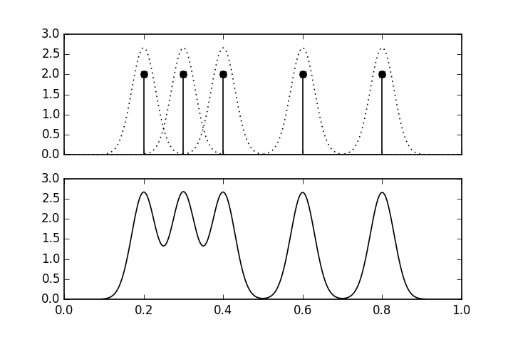
# where $X\in \mathbb{R}^d$. [Figure](#fig:nonparametric_002) shows an
# example of
# a kernel density estimate using a Gaussian kernel function,
# $K(x)=e^{-x^2/2}/\sqrt{2\pi}$. There are five data points shown by the
# vertical
# lines in the upper panel. The dotted lines show the individual $K(x)$
# function
# at each of the data points. The lower panel shows the overall kernel
# density
# estimate, which is the scaled sum of the upper panel.
#
# There is an important
# technical result in [[wasserman2004all]](#wasserman2004all) that
# states that
# kernel density estimators are minimax in the sense we
# discussed in the maximum
# likelihood the section [ch:stats:sec:mle](#ch:stats:sec:mle). In
# broad strokes,
# this means that the analogous risk for the kernel
# density estimator is
# approximately bounded by the following factor,
#
# $$
# R(p,\hat{p}) \lesssim n^{-\frac{2 m}{2 m+d}}
# $$
#
# for some constant $C$ where $m$ is a factor related to bounding
# the derivatives
# of the probability density function. For example, if the second
# derivative of
# the density function is bounded, then $m=2$. This means that
# the convergence
# rate for this estimator decreases with increasing dimension
# $d$.
#
#
#
#
#
#
#
#
#
#
# ## Kernel Smoothing
#
# We can extend our methods
# to other function classes using kernel functions.
# A one-dimensional smoothing
# kernel is a smooth function $K$ with
# the following properties,
#
# $$
# \begin{align*}
# \int K(x) dx &= 1 \\\
# \int x K(x) dx &= 0 \\\
# 0< \int x^2 K(x)
# dx &< \infty \\\
# \end{align*}
# $$
#
# For example, $K(x)=I(x)/2$ is the boxcar kernel, where $I(x)=1$
# when $\vert
# x\vert\le 1$ and zero otherwise. The kernel density estimator is
# very similar to
# the histogram, except now we put a kernel function on every
# point as in the
# following,
#
# $$
# \hat{p}(x)=\frac{1}{n}\sum_{i=1}^n \frac{1}{h^d} K\left(\frac{\Vert
# x-X_i\Vert}{h}\right)
# $$
#
# where $X\in \mathbb{R}^d$. [Figure](#fig:nonparametric_002) shows an
# example of
# a kernel density estimate using a Gaussian kernel function,
# $K(x)=e^{-x^2/2}/\sqrt{2\pi}$. There are five data points shown by the
# vertical
# lines in the upper panel. The dotted lines show the individual $K(x)$
# function
# at each of the data points. The lower panel shows the overall kernel
# density
# estimate, which is the scaled sum of the upper panel.
#
# There is an important
# technical result in [[wasserman2004all]](#wasserman2004all) that
# states that
# kernel density estimators are minimax in the sense we
# discussed in the maximum
# likelihood the section [ch:stats:sec:mle](#ch:stats:sec:mle). In
# broad strokes,
# this means that the analogous risk for the kernel
# density estimator is
# approximately bounded by the following factor,
#
# $$
# R(p,\hat{p}) \lesssim n^{-\frac{2 m}{2 m+d}}
# $$
#
# for some constant $C$ where $m$ is a factor related to bounding
# the derivatives
# of the probability density function. For example, if the second
# derivative of
# the density function is bounded, then $m=2$. This means that
# the convergence
# rate for this estimator decreases with increasing dimension
# $d$.
#
#
#
#
#
# The upper panel shows the individual # kernel functions placed at each of the data points. The lower panel shows the # composite kernel density estimate which is the sum of the individual functions # in the upper panel.
# #
#
#
#
# ### Cross-Validation
#
# As a practical matter,
# the tricky part of the kernel density estimator (which
# includes the histogram as
# a special case) is that we need to somehow compute
# the bandwidth $h$ term using
# data. There are several rule-of-thumb methods that
# for some common kernels,
# including Silverman's rule and Scott's rule for
# Gaussian kernels. For example,
# Scott's factor is to simply compute $h=n^{
# -1/(d+4) }$ and Silverman's is $h=(n
# (d+2)/4)^{ (-1/(d+4)) }$. Rules of
# this kind are derived by assuming the
# underlying probability density
# function is of a certain family (e.g., Gaussian),
# and then deriving the
# best $h$ for a certain type of kernel density estimator,
# usually equipped
# with extra functional properties (say, continuous derivatives
# of a
# certain order). In practice, these rules seem to work pretty well,
# especially for uni-modal probability density functions. Avoiding these
# kinds of
# assumptions means computing the bandwidth from data directly and that is where
# cross validation comes in.
#
# Cross-validation is a method to estimate the
# bandwidth from the data itself.
# The idea is to write out the following
# Integrated Squared Error (ISE),
#
# $$
# \begin{align*}
# \textnormal{ISE}(\hat{p}_h,p)&=\int (p(x)-\hat{p}_h(x))^2
# dx\\\
# &= \int \hat{p}_h(x)^2 dx - 2\int p(x)
# \hat{p}_h dx + \int p(x)^2 dx
# \end{align*}
# $$
#
# The problem with this expression is the middle term [^last_term],
# [^last_term]: The last term is of no interest because we are
# only interested in
# relative changes in the ISE.
#
# $$
# \int p(x)\hat{p}_h dx
# $$
#
# where $p(x)$ is what we are trying to estimate with $\hat{p}_h$. The
# form of
# the last expression looks like an expectation of $\hat{p}_h$ over the
# density of
# $p(x)$, $\mathbb{E}(\hat{p}_h)$. The approach is to
# approximate this with the
# mean,
#
# $$
# \mathbb{E}(\hat{p}_h) \approx \frac{1}{n}\sum_{i=1}^n \hat{p}_h(X_i)
# $$
#
# The problem with this approach is that $\hat{p}_h$ is computed using
# the same
# data that the approximation utilizes. The way to get around this is
# to split
# the data into two equally sized chunks $D_1$, $D_2$; and then compute
# $\hat{p}_h$ for a sequence of different $h$ values over the $D_1$ set. Then,
# when we apply the above approximation for the data ($Z_i$) in the $D_2$ set,
#
# $$
# \mathbb{E}(\hat{p}_h) \approx \frac{1}{\vert D_2\vert}\sum_{Z_i\in D_2}
# \hat{p}_h(Z_i)
# $$
#
# Plugging this approximation back into the integrated squared error
# provides
# the objective function,
#
# $$
# \texttt{ISE}\approx \int \hat{p}_h(x)^2 dx-\frac{2}{\vert
# D_2\vert}\sum_{Z_i\in D_2} \hat{p}_h(Z_i)
# $$
#
# Some code will make these steps concrete. We will need some tools from
# Scikit-
# learn.
# In[3]:
from sklearn.model_selection import train_test_split
from sklearn.neighbors.kde import KernelDensity
# The `train_test_split` function makes it easy to split and
# keep track of the
# $D_1$ and $D_2$ sets we need for cross validation. Scikit-learn
# already has a
# powerful and flexible implementation of kernel density estimators.
# To compute
# the objective function, we need some
# basic numerical integration tools from
# Scipy. For this example, we
# will generate samples from a $\beta(2,2)$
# distribution, which is
# implemented in the `stats` submodule in Scipy.
# In[4]:
import numpy as np
np.random.seed(123456)
# In[5]:
from scipy.integrate import quad
from scipy import stats
rv= stats.beta(2,2)
n=100 # number of samples to generate
d = rv.rvs(n)[:,None] # generate samples as column-vector
# **Programming Tip.**
#
# The use of the `[:,None]` in the last line formats the
# Numpy array returned by
# the `rvs` function into a Numpy vector with a column
# dimension of one. This is
# required by the `KernelDensity` constructor because
# the column dimension is
# used for different features (in general) for Scikit-
# learn. Thus, even though we
# only have one feature, we still need to comply with
# the structured input that
# Scikit-learn relies upon. There are many ways to
# inject the additional
# dimension other than using `None`. For example, the more
# cryptic, `np.c_`, or
# the less cryptic `[:,np.newaxis]` can do the same, as can
# the `np.reshape`
# function.
#
#
#
# The next step is to split the data into two
# halves and loop over
# each of the $h_i$ bandwidths to create a separate kernel
# density estimator
# based on the $D_1$ data,
# In[6]:
train,test,_,_=train_test_split(d,d,test_size=0.5)
kdes=[KernelDensity(bandwidth=i).fit(train)
for i in [.05,0.1,0.2,0.3]]
# **Programming Tip.**
#
# Note that the single underscore symbol in Python refers to
# the last evaluated
# result. the above code unpacks the tuple returned by
# `train_test_split` into
# four elements. Because we are only interested in the
# first two, we assign the
# last two to the underscore symbol. This is a stylistic
# usage to make it clear
# to the reader that the last two elements of the tuple are
# unused.
# Alternatively, we could assign the last two elements to a pair of dummy
# variables that we do not use later, but then the reader skimming the code may
# think that those dummy variables are relevant.
#
#
#
# The last step is to loop over
# the so-created kernel density estimators
# and compute the objective function.
# In[7]:
for i in kdes:
f = lambda x: np.exp(i.score_samples(x))
f2 = lambda x: f([[x]])**2
print('h=%3.2f\t %3.4f'%(i.bandwidth,quad(f2,0,1)[0]
-2*np.mean(f(test))))
# **Programming Tip.**
#
# The lambda functions defined in the last block are
# necessary because
# Scikit-learn implements the return value of the kernel density
# estimator as a
# logarithm via the `score_samples` function. The numerical
# quadrature function
# `quad` from Scipy computes the $\int \hat{p}_h(x)^2 dx$ part
# of the objective
# function.
# In[8]:
get_ipython().run_line_magic('matplotlib', 'inline')
# In[9]:
from __future__ import division
from matplotlib.pylab import subplots
fig,ax=subplots()
xi = np.linspace(0,1,100)[:,None]
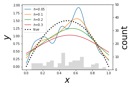
for i in kdes:
f=lambda x: np.exp(i.score_samples(x))
f2 = lambda x: f(x)**2
_=ax.plot(xi,f(xi),label='$h$='+str(i.bandwidth))
_=ax.set_xlabel('$x$',fontsize=28)
_=ax.set_ylabel('$y$',fontsize=28)
_=ax.plot(xi,rv.pdf(xi),'k:',lw=3,label='true')
_=ax.legend(loc=0)
ax2 = ax.twinx()
_=ax2.hist(d,20,alpha=.3,color='gray')
_=ax2.axis(ymax=50)
_=ax2.set_ylabel('count',fontsize=28)
fig.tight_layout()
fig.savefig('fig-statistics/nonparametric_003.png')
#
#
#
#
#
#
#
#
#
# ### Cross-Validation
#
# As a practical matter,
# the tricky part of the kernel density estimator (which
# includes the histogram as
# a special case) is that we need to somehow compute
# the bandwidth $h$ term using
# data. There are several rule-of-thumb methods that
# for some common kernels,
# including Silverman's rule and Scott's rule for
# Gaussian kernels. For example,
# Scott's factor is to simply compute $h=n^{
# -1/(d+4) }$ and Silverman's is $h=(n
# (d+2)/4)^{ (-1/(d+4)) }$. Rules of
# this kind are derived by assuming the
# underlying probability density
# function is of a certain family (e.g., Gaussian),
# and then deriving the
# best $h$ for a certain type of kernel density estimator,
# usually equipped
# with extra functional properties (say, continuous derivatives
# of a
# certain order). In practice, these rules seem to work pretty well,
# especially for uni-modal probability density functions. Avoiding these
# kinds of
# assumptions means computing the bandwidth from data directly and that is where
# cross validation comes in.
#
# Cross-validation is a method to estimate the
# bandwidth from the data itself.
# The idea is to write out the following
# Integrated Squared Error (ISE),
#
# $$
# \begin{align*}
# \textnormal{ISE}(\hat{p}_h,p)&=\int (p(x)-\hat{p}_h(x))^2
# dx\\\
# &= \int \hat{p}_h(x)^2 dx - 2\int p(x)
# \hat{p}_h dx + \int p(x)^2 dx
# \end{align*}
# $$
#
# The problem with this expression is the middle term [^last_term],
# [^last_term]: The last term is of no interest because we are
# only interested in
# relative changes in the ISE.
#
# $$
# \int p(x)\hat{p}_h dx
# $$
#
# where $p(x)$ is what we are trying to estimate with $\hat{p}_h$. The
# form of
# the last expression looks like an expectation of $\hat{p}_h$ over the
# density of
# $p(x)$, $\mathbb{E}(\hat{p}_h)$. The approach is to
# approximate this with the
# mean,
#
# $$
# \mathbb{E}(\hat{p}_h) \approx \frac{1}{n}\sum_{i=1}^n \hat{p}_h(X_i)
# $$
#
# The problem with this approach is that $\hat{p}_h$ is computed using
# the same
# data that the approximation utilizes. The way to get around this is
# to split
# the data into two equally sized chunks $D_1$, $D_2$; and then compute
# $\hat{p}_h$ for a sequence of different $h$ values over the $D_1$ set. Then,
# when we apply the above approximation for the data ($Z_i$) in the $D_2$ set,
#
# $$
# \mathbb{E}(\hat{p}_h) \approx \frac{1}{\vert D_2\vert}\sum_{Z_i\in D_2}
# \hat{p}_h(Z_i)
# $$
#
# Plugging this approximation back into the integrated squared error
# provides
# the objective function,
#
# $$
# \texttt{ISE}\approx \int \hat{p}_h(x)^2 dx-\frac{2}{\vert
# D_2\vert}\sum_{Z_i\in D_2} \hat{p}_h(Z_i)
# $$
#
# Some code will make these steps concrete. We will need some tools from
# Scikit-
# learn.
# In[3]:
from sklearn.model_selection import train_test_split
from sklearn.neighbors.kde import KernelDensity
# The `train_test_split` function makes it easy to split and
# keep track of the
# $D_1$ and $D_2$ sets we need for cross validation. Scikit-learn
# already has a
# powerful and flexible implementation of kernel density estimators.
# To compute
# the objective function, we need some
# basic numerical integration tools from
# Scipy. For this example, we
# will generate samples from a $\beta(2,2)$
# distribution, which is
# implemented in the `stats` submodule in Scipy.
# In[4]:
import numpy as np
np.random.seed(123456)
# In[5]:
from scipy.integrate import quad
from scipy import stats
rv= stats.beta(2,2)
n=100 # number of samples to generate
d = rv.rvs(n)[:,None] # generate samples as column-vector
# **Programming Tip.**
#
# The use of the `[:,None]` in the last line formats the
# Numpy array returned by
# the `rvs` function into a Numpy vector with a column
# dimension of one. This is
# required by the `KernelDensity` constructor because
# the column dimension is
# used for different features (in general) for Scikit-
# learn. Thus, even though we
# only have one feature, we still need to comply with
# the structured input that
# Scikit-learn relies upon. There are many ways to
# inject the additional
# dimension other than using `None`. For example, the more
# cryptic, `np.c_`, or
# the less cryptic `[:,np.newaxis]` can do the same, as can
# the `np.reshape`
# function.
#
#
#
# The next step is to split the data into two
# halves and loop over
# each of the $h_i$ bandwidths to create a separate kernel
# density estimator
# based on the $D_1$ data,
# In[6]:
train,test,_,_=train_test_split(d,d,test_size=0.5)
kdes=[KernelDensity(bandwidth=i).fit(train)
for i in [.05,0.1,0.2,0.3]]
# **Programming Tip.**
#
# Note that the single underscore symbol in Python refers to
# the last evaluated
# result. the above code unpacks the tuple returned by
# `train_test_split` into
# four elements. Because we are only interested in the
# first two, we assign the
# last two to the underscore symbol. This is a stylistic
# usage to make it clear
# to the reader that the last two elements of the tuple are
# unused.
# Alternatively, we could assign the last two elements to a pair of dummy
# variables that we do not use later, but then the reader skimming the code may
# think that those dummy variables are relevant.
#
#
#
# The last step is to loop over
# the so-created kernel density estimators
# and compute the objective function.
# In[7]:
for i in kdes:
f = lambda x: np.exp(i.score_samples(x))
f2 = lambda x: f([[x]])**2
print('h=%3.2f\t %3.4f'%(i.bandwidth,quad(f2,0,1)[0]
-2*np.mean(f(test))))
# **Programming Tip.**
#
# The lambda functions defined in the last block are
# necessary because
# Scikit-learn implements the return value of the kernel density
# estimator as a
# logarithm via the `score_samples` function. The numerical
# quadrature function
# `quad` from Scipy computes the $\int \hat{p}_h(x)^2 dx$ part
# of the objective
# function.
# In[8]:
get_ipython().run_line_magic('matplotlib', 'inline')
# In[9]:
from __future__ import division
from matplotlib.pylab import subplots
fig,ax=subplots()
xi = np.linspace(0,1,100)[:,None]
for i in kdes:
f=lambda x: np.exp(i.score_samples(x))
f2 = lambda x: f(x)**2
_=ax.plot(xi,f(xi),label='$h$='+str(i.bandwidth))
_=ax.set_xlabel('$x$',fontsize=28)
_=ax.set_ylabel('$y$',fontsize=28)
_=ax.plot(xi,rv.pdf(xi),'k:',lw=3,label='true')
_=ax.legend(loc=0)
ax2 = ax.twinx()
_=ax2.hist(d,20,alpha=.3,color='gray')
_=ax2.axis(ymax=50)
_=ax2.set_ylabel('count',fontsize=28)
fig.tight_layout()
fig.savefig('fig-statistics/nonparametric_003.png')
#
#
#
#
# Each line above is a # different kernel density estimator for the given bandwidth as an approximation # to the true density function. A plain histogram is imprinted on the bottom for # reference.
# #
#
#
#
# Scikit-learn has many more advanced tools to automate this kind
# of
# hyper-parameter (i.e., kernel density bandwidth) search. To utilize these
# advanced tools, we need to format the current problem slightly differently by
# defining the following wrapper class.
# In[10]:
class KernelDensityWrapper(KernelDensity):
def predict(self,x):
return np.exp(self.score_samples(x))
def score(self,test):
f = lambda x: self.predict(x)
f2 = lambda x: f([[x]])**2
return -(quad(f2,0,1)[0]-2*np.mean(f(test)))
# This is tantamount to reorganizing the above previous code
# into functions that
# Scikit-learn requires. Next, we create the
# dictionary of parameters we want to
# search over (`params`) below
# and then start the grid search with the `fit`
# function,
# In[11]:
from sklearn.model_selection import GridSearchCV
params = {'bandwidth':np.linspace(0.01,0.5,10)}
clf = GridSearchCV(KernelDensityWrapper(), param_grid=params,cv=2)
clf.fit(d)
print (clf.best_params_)
# The grid search iterates over all the elements in the `params`
# dictionary and
# reports the best bandwidth over that list of parameter values.
# The `cv` keyword
# argument above specifies that we want to split the data
# into two equally-sized
# sets for training and testing. We can
# also examine the values of the objective
# function for each point
# on the grid as follow,
# In[12]:
clf.cv_results_['mean_test_score']
# Keep in mind that the grid search examines multiple folds for cross
# validation
# to compute the above means and standard deviations. Note that there
# is also a
# `RandomizedSearchCV` in case you would rather specify a distribution
# of
# parameters instead of a list. This is particularly useful for searching very
# large parameter spaces where an exhaustive grid search would be too
# computationally expensive. Although kernel density estimators are easy to
# understand and have many attractive analytical properties, they become
# practically prohibitive for large, high-dimensional data sets.
#
# ## Nonparametric
# Regression Estimators
#
# Beyond estimating the underlying probability density, we
# can use nonparametric
# methods to compute estimators of the underlying function
# that is generating the
# data. Nonparametric regression estimators of the
# following form are known as
# linear smoothers,
#
# $$
# \hat{y}(x) = \sum_{i=1}^n \ell_i(x) y_i
# $$
#
# To understand the performance of these smoothers,
# we can define the risk as the
# following,
#
# $$
# R(\hat{y},y) = \mathbb{E}\left( \frac{1}{n} \sum_{i=1}^n
# (\hat{y}(x_i)-y(x_i))^2 \right)
# $$
#
# and find the best $\hat{y}$ that minimizes this. The problem with
# this metric
# is that we do not know $y(x)$, which is why we are trying to
# approximate it with
# $\hat{y}(x)$. We could construct an estimation by using the
# data at hand as in
# the following,
#
# $$
# \hat{R}(\hat{y},y) =\frac{1}{n} \sum_{i=1}^n (\hat{y}(x_i)-Y_i)^2
# $$
#
# where we have substituted the data $Y_i$ for the unknown function
# value,
# $y(x_i)$. The problem with this approach is that we are using the data
# to
# estimate the function and then using the same data to evaluate the risk of
# doing
# so. This kind of double-dipping leads to overly optimistic estimators.
# One way
# out of this conundrum is to use leave-one-out cross validation, wherein
# the
# $\hat{y}$ function is estimated using all but one of the data pairs,
# $(X_i,Y_i)$. Then, this missing data element is used to estimate the above
# risk.
# Notationally, this is written as the following,
#
# $$
# \hat{R}(\hat{y},y) =\frac{1}{n} \sum_{i=1}^n (\hat{y}_{(-i)}(x_i)-Y_i)^2
# $$
#
# where $\hat{y}_{(-i)}$ denotes computing the estimator without using
# the
# $i^{th}$ data pair. Unfortunately, for anything other than relatively small
# data
# sets, it quickly becomes computationally prohibitive to use leave-one-out
# cross
# validation in practice. We'll get back to this issue shortly, but let's
# consider
# a concrete example of such a nonparametric smoother.
#
# ## Nearest Neighbors
# Regression
#
#
# The simplest possible
# nonparametric regression method is the $k$-nearest
# neighbors regression. This is
# easier to explain in words than to write out in
# math. Given an input $x$, find
# the closest one of the $k$ clusters that
# contains it and then return the mean of
# the data values in that cluster. As a
# univariate example, let's consider the
# following *chirp* waveform,
#
# $$
# y(x)=\cos\left(2\pi\left(f_o x + \frac{BW x^2}{2\tau}\right)\right)
# $$
#
# This waveform is important in high-resolution radar applications.
# The $f_o$ is
# the start frequency and $BW/\tau$ is the frequency slope of the
# signal. For our
# example, the fact that it is nonuniform over its domain is
# important. We can
# easily create some data by sampling the
# chirp as in the following,
# In[13]:
from numpy import cos, pi
xi = np.linspace(0,1,100)[:,None]
xin = np.linspace(0,1,12)[:,None]
f0 = 1 # init frequency
BW = 5
y = np.cos(2*pi*(f0*xin+(BW/2.0)*xin**2))
# We can use this data to construct a simple nearest neighbor
# estimator using
# Scikit-learn,
# In[14]:
from sklearn.neighbors import KNeighborsRegressor
knr=KNeighborsRegressor(2)
knr.fit(xin,y)
# **Programming Tip.**
#
# Scikit-learn has a fantastically consistent interface. The
# `fit` function above
# fits the model parameters to the data. The corresponding
# `predict` function
# returns the output of the model given an arbitrary input. We
# will spend a lot
# more time on Scikit-learn in the machine learning chapter. The
# `[:,None]` part
# at the end is just injecting a column dimension into the array
# in order to
# satisfy the dimensional requirements of Scikit-learn.
# In[15]:
from matplotlib.pylab import subplots
fig,ax=subplots()
yi = cos(2*pi*(f0*xi+(BW/2.0)*xi**2))
_=ax.plot(xi,yi,'k--',lw=2,label=r'$y(x)$')
_=ax.plot(xin,y,'ko',lw=2,ms=11,color='gray',alpha=.8,label='$y(x_i)$')
_=ax.fill_between(xi.flat,yi.flat,knr.predict(xi).flat,color='gray',alpha=.3)
_=ax.plot(xi,knr.predict(xi),'k-',lw=2,label='$\hat{y}(x)$')
_=ax.set_aspect(1/4.)
_=ax.axis(ymax=1.05,ymin=-1.05)
_=ax.set_xlabel(r'$x$',fontsize=24)
_=ax.legend(loc=0)
fig.set_tight_layout(True)
fig.savefig('fig-statistics/nonparametric_004.png')
#
#
#
#
#
#
#
#
#
# Scikit-learn has many more advanced tools to automate this kind
# of
# hyper-parameter (i.e., kernel density bandwidth) search. To utilize these
# advanced tools, we need to format the current problem slightly differently by
# defining the following wrapper class.
# In[10]:
class KernelDensityWrapper(KernelDensity):
def predict(self,x):
return np.exp(self.score_samples(x))
def score(self,test):
f = lambda x: self.predict(x)
f2 = lambda x: f([[x]])**2
return -(quad(f2,0,1)[0]-2*np.mean(f(test)))
# This is tantamount to reorganizing the above previous code
# into functions that
# Scikit-learn requires. Next, we create the
# dictionary of parameters we want to
# search over (`params`) below
# and then start the grid search with the `fit`
# function,
# In[11]:
from sklearn.model_selection import GridSearchCV
params = {'bandwidth':np.linspace(0.01,0.5,10)}
clf = GridSearchCV(KernelDensityWrapper(), param_grid=params,cv=2)
clf.fit(d)
print (clf.best_params_)
# The grid search iterates over all the elements in the `params`
# dictionary and
# reports the best bandwidth over that list of parameter values.
# The `cv` keyword
# argument above specifies that we want to split the data
# into two equally-sized
# sets for training and testing. We can
# also examine the values of the objective
# function for each point
# on the grid as follow,
# In[12]:
clf.cv_results_['mean_test_score']
# Keep in mind that the grid search examines multiple folds for cross
# validation
# to compute the above means and standard deviations. Note that there
# is also a
# `RandomizedSearchCV` in case you would rather specify a distribution
# of
# parameters instead of a list. This is particularly useful for searching very
# large parameter spaces where an exhaustive grid search would be too
# computationally expensive. Although kernel density estimators are easy to
# understand and have many attractive analytical properties, they become
# practically prohibitive for large, high-dimensional data sets.
#
# ## Nonparametric
# Regression Estimators
#
# Beyond estimating the underlying probability density, we
# can use nonparametric
# methods to compute estimators of the underlying function
# that is generating the
# data. Nonparametric regression estimators of the
# following form are known as
# linear smoothers,
#
# $$
# \hat{y}(x) = \sum_{i=1}^n \ell_i(x) y_i
# $$
#
# To understand the performance of these smoothers,
# we can define the risk as the
# following,
#
# $$
# R(\hat{y},y) = \mathbb{E}\left( \frac{1}{n} \sum_{i=1}^n
# (\hat{y}(x_i)-y(x_i))^2 \right)
# $$
#
# and find the best $\hat{y}$ that minimizes this. The problem with
# this metric
# is that we do not know $y(x)$, which is why we are trying to
# approximate it with
# $\hat{y}(x)$. We could construct an estimation by using the
# data at hand as in
# the following,
#
# $$
# \hat{R}(\hat{y},y) =\frac{1}{n} \sum_{i=1}^n (\hat{y}(x_i)-Y_i)^2
# $$
#
# where we have substituted the data $Y_i$ for the unknown function
# value,
# $y(x_i)$. The problem with this approach is that we are using the data
# to
# estimate the function and then using the same data to evaluate the risk of
# doing
# so. This kind of double-dipping leads to overly optimistic estimators.
# One way
# out of this conundrum is to use leave-one-out cross validation, wherein
# the
# $\hat{y}$ function is estimated using all but one of the data pairs,
# $(X_i,Y_i)$. Then, this missing data element is used to estimate the above
# risk.
# Notationally, this is written as the following,
#
# $$
# \hat{R}(\hat{y},y) =\frac{1}{n} \sum_{i=1}^n (\hat{y}_{(-i)}(x_i)-Y_i)^2
# $$
#
# where $\hat{y}_{(-i)}$ denotes computing the estimator without using
# the
# $i^{th}$ data pair. Unfortunately, for anything other than relatively small
# data
# sets, it quickly becomes computationally prohibitive to use leave-one-out
# cross
# validation in practice. We'll get back to this issue shortly, but let's
# consider
# a concrete example of such a nonparametric smoother.
#
# ## Nearest Neighbors
# Regression
#
#
# The simplest possible
# nonparametric regression method is the $k$-nearest
# neighbors regression. This is
# easier to explain in words than to write out in
# math. Given an input $x$, find
# the closest one of the $k$ clusters that
# contains it and then return the mean of
# the data values in that cluster. As a
# univariate example, let's consider the
# following *chirp* waveform,
#
# $$
# y(x)=\cos\left(2\pi\left(f_o x + \frac{BW x^2}{2\tau}\right)\right)
# $$
#
# This waveform is important in high-resolution radar applications.
# The $f_o$ is
# the start frequency and $BW/\tau$ is the frequency slope of the
# signal. For our
# example, the fact that it is nonuniform over its domain is
# important. We can
# easily create some data by sampling the
# chirp as in the following,
# In[13]:
from numpy import cos, pi
xi = np.linspace(0,1,100)[:,None]
xin = np.linspace(0,1,12)[:,None]
f0 = 1 # init frequency
BW = 5
y = np.cos(2*pi*(f0*xin+(BW/2.0)*xin**2))
# We can use this data to construct a simple nearest neighbor
# estimator using
# Scikit-learn,
# In[14]:
from sklearn.neighbors import KNeighborsRegressor
knr=KNeighborsRegressor(2)
knr.fit(xin,y)
# **Programming Tip.**
#
# Scikit-learn has a fantastically consistent interface. The
# `fit` function above
# fits the model parameters to the data. The corresponding
# `predict` function
# returns the output of the model given an arbitrary input. We
# will spend a lot
# more time on Scikit-learn in the machine learning chapter. The
# `[:,None]` part
# at the end is just injecting a column dimension into the array
# in order to
# satisfy the dimensional requirements of Scikit-learn.
# In[15]:
from matplotlib.pylab import subplots
fig,ax=subplots()
yi = cos(2*pi*(f0*xi+(BW/2.0)*xi**2))
_=ax.plot(xi,yi,'k--',lw=2,label=r'$y(x)$')
_=ax.plot(xin,y,'ko',lw=2,ms=11,color='gray',alpha=.8,label='$y(x_i)$')
_=ax.fill_between(xi.flat,yi.flat,knr.predict(xi).flat,color='gray',alpha=.3)
_=ax.plot(xi,knr.predict(xi),'k-',lw=2,label='$\hat{y}(x)$')
_=ax.set_aspect(1/4.)
_=ax.axis(ymax=1.05,ymin=-1.05)
_=ax.set_xlabel(r'$x$',fontsize=24)
_=ax.legend(loc=0)
fig.set_tight_layout(True)
fig.savefig('fig-statistics/nonparametric_004.png')
#
#
#
#
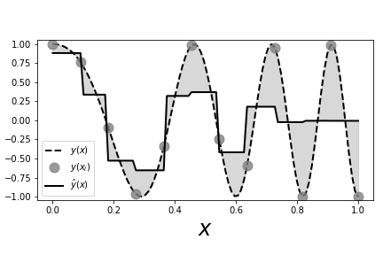
# The dotted line shows the chirp # signal and the solid line shows the nearest neighbor estimate. The gray circles # are the sample points that we used to fit the nearest neighbor estimator. The # shaded area shows the gaps between the estimator and the unsampled chirp.
# #
#
# [Figure](#fig:nonparametric_004) shows the sampled signal (gray
# circles) against
# the values generated by the nearest neighbor estimator (solid
# line). The dotted
# line is the full unsampled chirp signal, which increases in
# frequency with $x$.
# This is important for our example because it adds a
# non-stationary aspect to
# this problem in that the function gets progressively
# wigglier with increasing
# $x$. The area between the estimated curve and the
# signal is shaded in gray.
# Because the nearest neighbor estimator uses only two
# nearest neighbors, for each
# new $x$, it finds the two adjacent $X_i$ that
# bracket the $x$ in the training
# data and then averages the corresponding $Y_i$
# values to compute the estimated
# value. That is, if you take every adjacent pair
# of sequential gray circles in
# the Figure, you find that the horizontal solid line
# splits the pair on the
# vertical axis. We can adjust the number of
# nearest neighbors by changing the
# constructor,
# In[16]:
knr=KNeighborsRegressor(3)
knr.fit(xin,y)
# In[17]:
fig,ax=subplots()
_=ax.plot(xi,yi,'k--',lw=2,label=r'$y(x)$')
_=ax.plot(xin,y,'ko',lw=2,ms=11,color='gray',alpha=.8,label='$y(x_i)$')
_=ax.fill_between(xi.flat,yi.flat,knr.predict(xi).flat,color='gray',alpha=.3)
_=ax.plot(xi,knr.predict(xi),'k-',lw=2,label='$\hat{y}(x)$')
_=ax.set_aspect(1/4.)
_=ax.axis(ymax=1.05,ymin=-1.05)
_=ax.set_xlabel(r'$x$',fontsize=24)
_=ax.legend(loc=0)
fig.set_tight_layout(True)
fig.savefig('fig-statistics/nonparametric_005.png')
# which produces the following corresponding [Figure](#fig:nonparametric_005).
#
#
#
#
#
#
#
# [Figure](#fig:nonparametric_004) shows the sampled signal (gray
# circles) against
# the values generated by the nearest neighbor estimator (solid
# line). The dotted
# line is the full unsampled chirp signal, which increases in
# frequency with $x$.
# This is important for our example because it adds a
# non-stationary aspect to
# this problem in that the function gets progressively
# wigglier with increasing
# $x$. The area between the estimated curve and the
# signal is shaded in gray.
# Because the nearest neighbor estimator uses only two
# nearest neighbors, for each
# new $x$, it finds the two adjacent $X_i$ that
# bracket the $x$ in the training
# data and then averages the corresponding $Y_i$
# values to compute the estimated
# value. That is, if you take every adjacent pair
# of sequential gray circles in
# the Figure, you find that the horizontal solid line
# splits the pair on the
# vertical axis. We can adjust the number of
# nearest neighbors by changing the
# constructor,
# In[16]:
knr=KNeighborsRegressor(3)
knr.fit(xin,y)
# In[17]:
fig,ax=subplots()
_=ax.plot(xi,yi,'k--',lw=2,label=r'$y(x)$')
_=ax.plot(xin,y,'ko',lw=2,ms=11,color='gray',alpha=.8,label='$y(x_i)$')
_=ax.fill_between(xi.flat,yi.flat,knr.predict(xi).flat,color='gray',alpha=.3)
_=ax.plot(xi,knr.predict(xi),'k-',lw=2,label='$\hat{y}(x)$')
_=ax.set_aspect(1/4.)
_=ax.axis(ymax=1.05,ymin=-1.05)
_=ax.set_xlabel(r'$x$',fontsize=24)
_=ax.legend(loc=0)
fig.set_tight_layout(True)
fig.savefig('fig-statistics/nonparametric_005.png')
# which produces the following corresponding [Figure](#fig:nonparametric_005).
#
#
#
#
# This is the same as # [Figure](#fig:nonparametric_004) except that here there are three nearest # neighbors used to build the estimator.
# #
#
#
#
# For this
# example, [Figure](#fig:nonparametric_005) shows that with
# more nearest neighbors
# the fit performs poorly, especially towards the end of
# the signal, where there
# is increasing variation, because the chirp is not
# uniformly continuous.
#
# Scikit-
# learn provides many tools for cross validation. The following code
# sets up the
# tools for leave-one-out cross validation,
# In[18]:
from sklearn.model_selection import LeaveOneOut
loo=LeaveOneOut()
# The `LeaveOneOut` object is an iterable that produces a set of
# disjoint indices
# of the data --- one for fitting the model (training set) and
# one for evaluating
# the model (testing set). The next block loops over the
# disjoint sets of
# training and test indicies iterates provided by the `loo`
# variable to evaluate
# the estimated risk, which is accumulated in the `out`
# list.
# In[19]:
out=[]
for train_index, test_index in loo.split(xin):
_=knr.fit(xin[train_index],y[train_index])
out.append((knr.predict(xi[test_index])-y[test_index])**2)
print( 'Leave-one-out Estimated Risk: ',np.mean(out),)
# The last line in the code above reports leave-one-out's estimated
# risk.
# Linear smoothers of this type can be rewritten in using the following matrix,
#
# $$
# \mathscr{S} = \left[ \ell_i(x_j) \right]_{i,j}
# $$
#
# so that
#
# $$
# \hat{\mathbf{y}} = \mathscr{S} \mathbf{y}
# $$
#
# where $\mathbf{y}=\left[Y_1,Y_2,\ldots,Y_n\right]\in \mathbb{R}^n$
# and $\hat{
# \mathbf{y}
# }=\left[\hat{y}(x_1),\hat{y}(x_2),\ldots,\hat{y}(x_n)\right]\in
# \mathbb{R}^n$.
# This leads to a quick way to approximate leave-one-out cross
# validation as the
# following,
#
# $$
# \hat{R}=\frac{1}{n}\sum_{i=1}^n\left(\frac{y_i-\hat{y}(x_i)}{1-\mathscr{S}_{i,i}}\right)^2
# $$
#
# However, this does not reproduce the approach in the code above
# because it
# assumes that each $\hat{y}_{(-i)}(x_i)$ is consuming one fewer
# nearest neighbor
# than $\hat{y}(x)$.
#
# We can get this $\mathscr{S}$ matrix from the `knr` object
# as in the following,
# In[20]:
_= knr.fit(xin,y) # fit on all data
S=(knr.kneighbors_graph(xin)).todense()/float(knr.n_neighbors)
# The `todense` part reformats the sparse matrix that is
# returned into a regular
# Numpy `matrix`. The following shows a subsection
# of this $\mathcal{S}$ matrix,
# In[21]:
print(S[:5,:5])
# The sub-blocks show the windows of the the `y` data that are being
# processed by
# the nearest neighbor estimator. For example,
# In[22]:
print(np.hstack([knr.predict(xin[:5]),(S*y)[:5]]))#columns match
# Or, more concisely checking all entries for approximate equality,
# In[23]:
np.allclose(knr.predict(xin),S*y)
# which shows that the results from the nearest neighbor
# object and the matrix
# multiply match.
#
# **Programming Tip.**
#
# Note that because we formatted the
# returned $\mathscr{S}$ as a Numpy matrix, we
# automatically get the matrix
# multiplication instead of default element-wise
# multiplication in the `S*y` term.
# ## Kernel Regression
#
# For estimating the probability density, we started with
# the histogram and moved
# to the more general kernel density estimate. Likewise,
# we can also extend
# regression from nearest neighbors to kernel-based regression
# using the
# *Nadaraya-Watson* kernel regression estimator. Given a bandwidth
# $h>0$, the
# kernel regression estimator is defined as the following,
#
# $$
# \hat{y}(x)=\frac{\sum_{i=1}^n K\left(\frac{x-x_i}{h}\right) Y_i}{\sum_{i=1}^n
# K \left( \frac{x-x_i}{h} \right)}
# $$
#
# Unfortunately, Scikit-learn does not implement this
# regression estimator;
# however, Jan Hendrik Metzen makes a compatible
# version available on
# `github.com`.
# In[24]:
import sys
sys.path.append('../src-statistics')
xin = np.linspace(0,1,20)[:,None]
y = cos(2*pi*(f0*xin+(BW/2.0)*xin**2)).flatten()
# In[25]:
from kernel_regression import KernelRegression
# This code makes it possible to internally optimize over the bandwidth
# parameter
# using leave-one-out cross validation by specifying a grid of
# potential bandwidth
# values (`gamma`), as in the following,
# In[26]:
kr = KernelRegression(gamma=np.linspace(6e3,7e3,500))
kr.fit(xin,y)
# [Figure](#fig:nonparametric_006) shows the kernel estimator (heavy
# black line)
# using the Gaussian kernel compared to the nearest neighbor
# estimator (solid
# light black line). As before, the data points are shown as
# circles.
# [Figure](#fig:nonparametric_006) shows that the kernel estimator can
# pick out
# the sharp peaks that are missed by the nearest neighbor estimator.
#
#
#
#
#
#
#
#
#
#
# For this
# example, [Figure](#fig:nonparametric_005) shows that with
# more nearest neighbors
# the fit performs poorly, especially towards the end of
# the signal, where there
# is increasing variation, because the chirp is not
# uniformly continuous.
#
# Scikit-
# learn provides many tools for cross validation. The following code
# sets up the
# tools for leave-one-out cross validation,
# In[18]:
from sklearn.model_selection import LeaveOneOut
loo=LeaveOneOut()
# The `LeaveOneOut` object is an iterable that produces a set of
# disjoint indices
# of the data --- one for fitting the model (training set) and
# one for evaluating
# the model (testing set). The next block loops over the
# disjoint sets of
# training and test indicies iterates provided by the `loo`
# variable to evaluate
# the estimated risk, which is accumulated in the `out`
# list.
# In[19]:
out=[]
for train_index, test_index in loo.split(xin):
_=knr.fit(xin[train_index],y[train_index])
out.append((knr.predict(xi[test_index])-y[test_index])**2)
print( 'Leave-one-out Estimated Risk: ',np.mean(out),)
# The last line in the code above reports leave-one-out's estimated
# risk.
# Linear smoothers of this type can be rewritten in using the following matrix,
#
# $$
# \mathscr{S} = \left[ \ell_i(x_j) \right]_{i,j}
# $$
#
# so that
#
# $$
# \hat{\mathbf{y}} = \mathscr{S} \mathbf{y}
# $$
#
# where $\mathbf{y}=\left[Y_1,Y_2,\ldots,Y_n\right]\in \mathbb{R}^n$
# and $\hat{
# \mathbf{y}
# }=\left[\hat{y}(x_1),\hat{y}(x_2),\ldots,\hat{y}(x_n)\right]\in
# \mathbb{R}^n$.
# This leads to a quick way to approximate leave-one-out cross
# validation as the
# following,
#
# $$
# \hat{R}=\frac{1}{n}\sum_{i=1}^n\left(\frac{y_i-\hat{y}(x_i)}{1-\mathscr{S}_{i,i}}\right)^2
# $$
#
# However, this does not reproduce the approach in the code above
# because it
# assumes that each $\hat{y}_{(-i)}(x_i)$ is consuming one fewer
# nearest neighbor
# than $\hat{y}(x)$.
#
# We can get this $\mathscr{S}$ matrix from the `knr` object
# as in the following,
# In[20]:
_= knr.fit(xin,y) # fit on all data
S=(knr.kneighbors_graph(xin)).todense()/float(knr.n_neighbors)
# The `todense` part reformats the sparse matrix that is
# returned into a regular
# Numpy `matrix`. The following shows a subsection
# of this $\mathcal{S}$ matrix,
# In[21]:
print(S[:5,:5])
# The sub-blocks show the windows of the the `y` data that are being
# processed by
# the nearest neighbor estimator. For example,
# In[22]:
print(np.hstack([knr.predict(xin[:5]),(S*y)[:5]]))#columns match
# Or, more concisely checking all entries for approximate equality,
# In[23]:
np.allclose(knr.predict(xin),S*y)
# which shows that the results from the nearest neighbor
# object and the matrix
# multiply match.
#
# **Programming Tip.**
#
# Note that because we formatted the
# returned $\mathscr{S}$ as a Numpy matrix, we
# automatically get the matrix
# multiplication instead of default element-wise
# multiplication in the `S*y` term.
# ## Kernel Regression
#
# For estimating the probability density, we started with
# the histogram and moved
# to the more general kernel density estimate. Likewise,
# we can also extend
# regression from nearest neighbors to kernel-based regression
# using the
# *Nadaraya-Watson* kernel regression estimator. Given a bandwidth
# $h>0$, the
# kernel regression estimator is defined as the following,
#
# $$
# \hat{y}(x)=\frac{\sum_{i=1}^n K\left(\frac{x-x_i}{h}\right) Y_i}{\sum_{i=1}^n
# K \left( \frac{x-x_i}{h} \right)}
# $$
#
# Unfortunately, Scikit-learn does not implement this
# regression estimator;
# however, Jan Hendrik Metzen makes a compatible
# version available on
# `github.com`.
# In[24]:
import sys
sys.path.append('../src-statistics')
xin = np.linspace(0,1,20)[:,None]
y = cos(2*pi*(f0*xin+(BW/2.0)*xin**2)).flatten()
# In[25]:
from kernel_regression import KernelRegression
# This code makes it possible to internally optimize over the bandwidth
# parameter
# using leave-one-out cross validation by specifying a grid of
# potential bandwidth
# values (`gamma`), as in the following,
# In[26]:
kr = KernelRegression(gamma=np.linspace(6e3,7e3,500))
kr.fit(xin,y)
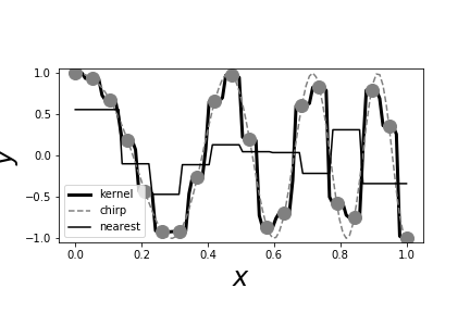
# [Figure](#fig:nonparametric_006) shows the kernel estimator (heavy
# black line)
# using the Gaussian kernel compared to the nearest neighbor
# estimator (solid
# light black line). As before, the data points are shown as
# circles.
# [Figure](#fig:nonparametric_006) shows that the kernel estimator can
# pick out
# the sharp peaks that are missed by the nearest neighbor estimator.
#
#
#
#
#
# The heavy black line is the Gaussian # kernel estimator. The light black line is the nearest neighbor estimator. The # data points are shown as gray circles. Note that unlike the nearest neighbor # estimator, the Gaussian kernel estimator is able to pick out the sharp peaks in # the training data.
# #
#
#
#
# Thus, the difference between nearest neighbor
# and kernel estimation is that the
# latter provides a smooth moving averaging of
# points whereas the former provides
# a discontinuous averaging. Note that kernel
# estimates suffer near the
# boundaries where there is mismatch between the edges
# and the kernel
# function. This problem gets worse in higher dimensions because
# the data
# naturally drift towards the boundaries (this is a consequence of the
# *curse of
# dimensionality*). Indeed, it is not possible to simultaneously
# maintain local
# accuracy (i.e., low bias) and a generous neighborhood (i.e., low
# variance). One
# way to address this problem is to create a local polynomial
# regression using
# the kernel function as a window to localize a region of
# interest. For example,
#
# $$
# \hat{y}(x)=\sum_{i=1}^n K\left(\frac{x-x_i}{h}\right) (Y_i-\alpha - \beta
# x_i)^2
# $$
#
# and now we have to optimize over the two linear parameters $\alpha$
# and
# $\beta$. This method is known as *local linear regression*
# [[loader2006local]](#loader2006local),
# [[hastie2013elements]](#hastie2013elements). Naturally, this can be
# extended to
# higher-order polynomials. Note that these methods are not yet
# implemented in
# Scikit-learn.
# In[27]:
fig,ax=subplots()
#fig.set_size_inches((12,4))
_=ax.plot(xi,kr.predict(xi),'k-',label='kernel',lw=3)
_=ax.plot(xin,y,'o',lw=3,color='gray',ms=12)
_=ax.plot(xi,yi,'--',color='gray',label='chirp')
_=ax.plot(xi,knr.predict(xi),'k-',label='nearest')
_=ax.axis(ymax=1.1,ymin=-1.1)
_=ax.set_aspect(1/4.)
_=ax.axis(ymax=1.05,ymin=-1.05)
_=ax.set_xlabel(r'$x$',fontsize=24)
_=ax.set_ylabel(r'$y$',fontsize=24)
_=ax.legend(loc=0)
fig.savefig('fig-statistics/nonparametric_006.png')
# ## Curse of Dimensionality
#
#
#
#
#
#
# The so-called curse of
# dimensionality occurs as we move into higher and higher
# dimensions. The term was
# coined by Bellman in 1961 while he was studying
# adaptive control processes.
# Nowadays, the term is vaguely refers to anything
# that becomes more complicated
# as the number of dimensions increases
# substantially. Nevertheless, the concept
# is useful for recognizing
# and characterizing the practical difficulties of high-
# dimensional analysis and
# estimation.
#
# Consider the volume of an $d$-dimensional
# sphere of radius $r$,
#
# $$
# V_s(d,r)=\frac{\pi ^{d/2} r^d}{\Gamma \left(\frac{d}{2}+1\right)}
# $$
#
# Further, consider the sphere $V_s(d,1/2)$ enclosed by an $d$
# dimensional unit
# cube. The volume of the cube is always equal to one, but
# $\lim_{d\rightarrow\infty} V_s(d,1/2) = 0$. What does this mean? It means that
# the volume of the cube is pushed away from its center, where the embedded
# hypersphere lives. Specifically, the distance from the center of the cube to
# its vertices in $d$ dimensions is $\sqrt{d}/2$, whereas the distance from the
# center of the inscribing sphere is $1/2$. This diagonal distance goes to
# infinity as $d$ does. For a fixed $d$, the tiny spherical region at the center
# of the cube has many long spines attached to it, like a hyper-dimensional sea
# urchin or porcupine.
#
# Another way to think about this is to consider the
# $\epsilon>0$ thick peel of the
# hypersphere,
#
# $$
# \mathcal{P}_{\epsilon} =V_s(d,r) - V_s(d,r-\epsilon)
# $$
#
# Then, we consider the following limit,
#
#
#
#
# $$
# \begin{equation}
# \lim_{d\rightarrow\infty}\mathcal{P}_{\epsilon}
# =\lim_{d\rightarrow\infty} V_s(d,r)\left(1 -
# \frac{V_s(d,r-\epsilon)}{V_s(d,r)}\right)
# \label{_auto1} \tag{1}
# \end{equation}
# $$
#
#
#
#
# $$
# \begin{equation} \
# =\lim_{d\rightarrow\infty} V_s(d,r)\left(1 -\lim_{d\rightarrow\infty}
# \left(\frac{r-\epsilon}{r}\right)^d\right)
# \label{_auto2} \tag{2}
# \end{equation}
# $$
#
#
#
#
# $$
# \begin{equation} \
# =\lim_{d\rightarrow\infty} V_s(d,r)
# \label{_auto3} \tag{3}
# \end{equation}
# $$
#
# So, in the limit, the volume of the $\epsilon$-thick peel
# consumes the volume
# of the hypersphere.
#
# What are the consequences of this? For methods that rely on
# nearest
# neighbors, exploiting locality to lower bias becomes intractable. For
# example, suppose we have an $d$ dimensional space and a point near the
# origin we
# want to localize around. To estimate behavior around this
# point, we need to
# average the unknown function about this point, but
# in a high-dimensional space,
# the chances of finding neighbors to
# average are slim. Looked at from the
# opposing point of view, suppose
# we have a binary variable, as in the coin-
# flipping problem. If we have
# 1000 trials, then, based on our earlier work, we
# can be confident
# about estimating the probability of heads. Now, suppose we
# have 10
# binary variables. Now we have $2^{ 10 }=1024$ vertices to estimate.
# If
# we had the same 1000 points, then at least 24 vertices would not
# get any data.
# To keep the same resolution, we would need 1000 samples
# at each vertex for a
# grand total of $1000\times 1024 \approx 10^6$
# data points. So, for a ten fold
# increase in the number of variables,
# we now have about 1000 more data points to
# collect to maintain the
# same statistical resolution. This is the curse of
# dimensionality.
#
# Perhaps some code will clarify this. The following code
# generates samples in
# two dimensions that are plotted as points in
# [Figure](#fig:curse_of_dimensionality_001) with the inscribed circle in two
# dimensions. Note that for $d=2$ dimensions, most of the points are contained
# in
# the circle.
# In[28]:
import numpy as np
v=np.random.rand(1000,2)-1/2.
# In[29]:
from matplotlib.patches import Circle
from matplotlib.pylab import subplots
fig,ax=subplots()
fig.set_size_inches((5,5))
_=ax.set_aspect(1)
_=ax.scatter(v[:,0],v[:,1],color='gray',alpha=.3)
_=ax.add_patch(Circle((0,0),0.5,alpha=.8,lw=3.,fill=False))
fig.savefig('fig-statistics/curse_of_dimensionality_001.pdf')
#
#
#
#
#
#
#
#
# Thus, the difference between nearest neighbor
# and kernel estimation is that the
# latter provides a smooth moving averaging of
# points whereas the former provides
# a discontinuous averaging. Note that kernel
# estimates suffer near the
# boundaries where there is mismatch between the edges
# and the kernel
# function. This problem gets worse in higher dimensions because
# the data
# naturally drift towards the boundaries (this is a consequence of the
# *curse of
# dimensionality*). Indeed, it is not possible to simultaneously
# maintain local
# accuracy (i.e., low bias) and a generous neighborhood (i.e., low
# variance). One
# way to address this problem is to create a local polynomial
# regression using
# the kernel function as a window to localize a region of
# interest. For example,
#
# $$
# \hat{y}(x)=\sum_{i=1}^n K\left(\frac{x-x_i}{h}\right) (Y_i-\alpha - \beta
# x_i)^2
# $$
#
# and now we have to optimize over the two linear parameters $\alpha$
# and
# $\beta$. This method is known as *local linear regression*
# [[loader2006local]](#loader2006local),
# [[hastie2013elements]](#hastie2013elements). Naturally, this can be
# extended to
# higher-order polynomials. Note that these methods are not yet
# implemented in
# Scikit-learn.
# In[27]:
fig,ax=subplots()
#fig.set_size_inches((12,4))
_=ax.plot(xi,kr.predict(xi),'k-',label='kernel',lw=3)
_=ax.plot(xin,y,'o',lw=3,color='gray',ms=12)
_=ax.plot(xi,yi,'--',color='gray',label='chirp')
_=ax.plot(xi,knr.predict(xi),'k-',label='nearest')
_=ax.axis(ymax=1.1,ymin=-1.1)
_=ax.set_aspect(1/4.)
_=ax.axis(ymax=1.05,ymin=-1.05)
_=ax.set_xlabel(r'$x$',fontsize=24)
_=ax.set_ylabel(r'$y$',fontsize=24)
_=ax.legend(loc=0)
fig.savefig('fig-statistics/nonparametric_006.png')
# ## Curse of Dimensionality
#
#
#
#
#
#
# The so-called curse of
# dimensionality occurs as we move into higher and higher
# dimensions. The term was
# coined by Bellman in 1961 while he was studying
# adaptive control processes.
# Nowadays, the term is vaguely refers to anything
# that becomes more complicated
# as the number of dimensions increases
# substantially. Nevertheless, the concept
# is useful for recognizing
# and characterizing the practical difficulties of high-
# dimensional analysis and
# estimation.
#
# Consider the volume of an $d$-dimensional
# sphere of radius $r$,
#
# $$
# V_s(d,r)=\frac{\pi ^{d/2} r^d}{\Gamma \left(\frac{d}{2}+1\right)}
# $$
#
# Further, consider the sphere $V_s(d,1/2)$ enclosed by an $d$
# dimensional unit
# cube. The volume of the cube is always equal to one, but
# $\lim_{d\rightarrow\infty} V_s(d,1/2) = 0$. What does this mean? It means that
# the volume of the cube is pushed away from its center, where the embedded
# hypersphere lives. Specifically, the distance from the center of the cube to
# its vertices in $d$ dimensions is $\sqrt{d}/2$, whereas the distance from the
# center of the inscribing sphere is $1/2$. This diagonal distance goes to
# infinity as $d$ does. For a fixed $d$, the tiny spherical region at the center
# of the cube has many long spines attached to it, like a hyper-dimensional sea
# urchin or porcupine.
#
# Another way to think about this is to consider the
# $\epsilon>0$ thick peel of the
# hypersphere,
#
# $$
# \mathcal{P}_{\epsilon} =V_s(d,r) - V_s(d,r-\epsilon)
# $$
#
# Then, we consider the following limit,
#
#
#
#
# $$
# \begin{equation}
# \lim_{d\rightarrow\infty}\mathcal{P}_{\epsilon}
# =\lim_{d\rightarrow\infty} V_s(d,r)\left(1 -
# \frac{V_s(d,r-\epsilon)}{V_s(d,r)}\right)
# \label{_auto1} \tag{1}
# \end{equation}
# $$
#
#
#
#
# $$
# \begin{equation} \
# =\lim_{d\rightarrow\infty} V_s(d,r)\left(1 -\lim_{d\rightarrow\infty}
# \left(\frac{r-\epsilon}{r}\right)^d\right)
# \label{_auto2} \tag{2}
# \end{equation}
# $$
#
#
#
#
# $$
# \begin{equation} \
# =\lim_{d\rightarrow\infty} V_s(d,r)
# \label{_auto3} \tag{3}
# \end{equation}
# $$
#
# So, in the limit, the volume of the $\epsilon$-thick peel
# consumes the volume
# of the hypersphere.
#
# What are the consequences of this? For methods that rely on
# nearest
# neighbors, exploiting locality to lower bias becomes intractable. For
# example, suppose we have an $d$ dimensional space and a point near the
# origin we
# want to localize around. To estimate behavior around this
# point, we need to
# average the unknown function about this point, but
# in a high-dimensional space,
# the chances of finding neighbors to
# average are slim. Looked at from the
# opposing point of view, suppose
# we have a binary variable, as in the coin-
# flipping problem. If we have
# 1000 trials, then, based on our earlier work, we
# can be confident
# about estimating the probability of heads. Now, suppose we
# have 10
# binary variables. Now we have $2^{ 10 }=1024$ vertices to estimate.
# If
# we had the same 1000 points, then at least 24 vertices would not
# get any data.
# To keep the same resolution, we would need 1000 samples
# at each vertex for a
# grand total of $1000\times 1024 \approx 10^6$
# data points. So, for a ten fold
# increase in the number of variables,
# we now have about 1000 more data points to
# collect to maintain the
# same statistical resolution. This is the curse of
# dimensionality.
#
# Perhaps some code will clarify this. The following code
# generates samples in
# two dimensions that are plotted as points in
# [Figure](#fig:curse_of_dimensionality_001) with the inscribed circle in two
# dimensions. Note that for $d=2$ dimensions, most of the points are contained
# in
# the circle.
# In[28]:
import numpy as np
v=np.random.rand(1000,2)-1/2.
# In[29]:
from matplotlib.patches import Circle
from matplotlib.pylab import subplots
fig,ax=subplots()
fig.set_size_inches((5,5))
_=ax.set_aspect(1)
_=ax.scatter(v[:,0],v[:,1],color='gray',alpha=.3)
_=ax.add_patch(Circle((0,0),0.5,alpha=.8,lw=3.,fill=False))
fig.savefig('fig-statistics/curse_of_dimensionality_001.pdf')
#
#
#
# Two dimensional scatter of points randomly and independently uniformly # distributed in the unit square. Note that most of the points are contained in # the circle. Counter to intuition, this does not persist as the number of # dimensions increases.
#Each panel shows the histogram # of lengths of uniformly distributed $d$ dimensional random vectors. The # population to the left of the dark vertical line are those that are contained in # the inscribed hypersphere. This shows that fewer points are contained in the # hypersphere with increasing dimension.
#The black line density function # is stochastically larger than the gray one.
# #
#
#
#
# ### The Mann-Whitney-Wilcoxon Test
#
# The Mann-Whitney-Wilcoxon Test approaches the
# following alternative hypotheses
#
# * $H_0$ : $F(x) = G(x)$ for all $x$ versus
# * $H_a$ : $F(x) \ge G(x)$, $F$ stochastically greater than $G$.
#
# Suppose we have
# two data sets $X$ and $Y$ and we want to know if they are drawn
# from the same
# underlying probability distribution or if one is stochastically
# greater than the
# other. There are $n_x$ elements in $X$ and $n_y$ elements in
# $Y$. If we combine
# these two data sets and rank them, then, under the null
# hypothesis, any data
# element should be as likely as any other to be assigned
# any particular rank.
# that is, the combined set $Z$,
#
# $$
# Z = \lbrace X_1,\ldots,X_{n_x}, Y_1,\ldots,Y_{n_y} \rbrace
# $$
#
# contains $n=n_x+n_y$ elements. Thus, any assignment of $n_y$ ranks
# from the
# integers $\lbrace 1,\ldots,n \rbrace$ to $\lbrace Y_1,\ldots,Y_{n_y}
# \rbrace$
# should be equally likely (i.e., $\mathbb{P}={ \binom{n}{n_y} }^{-1}$).
# Importantly, this property is independent of the $F$ distribution.
#
# That is, we
# can define the $U$ statistic as the following,
#
# $$
# U_X =\sum_{i=1}^{n_x}\sum_{j=1}^{n_y}\mathbb{I}(X_i\ge Y_j)
# $$
#
# where $\mathbb{I}(\cdot)$ is the usual indicator function. For an
# interpretation, this counts the number of times that elements of $Y$ outrank
# elements of $X$. For example, let us suppose that $X=\lbrace 1,3,4,5,6
# \rbrace$ and $Y=\lbrace 2,7,8,10,11 \rbrace$. We can get a this in one move
# using Numpy broadcasting,
# In[33]:
import numpy as np
x = np.array([ 1,3,4,5,6 ])
y = np.array([2,7,8,10,11])
U_X = (y <= x[:,None]).sum()
U_Y = (x <= y[:,None]).sum()
print (U_X, U_Y)
# Note that
#
# $$
# U_X+U_Y =\sum_{i=1}^{n_x}\sum_{j=1}^{n_y} \mathbb{I}(Y_i\ge
# X_j)+\mathbb{I}(X_i\ge Y_j)= n_x n_y
# $$
#
# because $\mathbb{I}(Y_i\ge X_j)+\mathbb{I}(X_i\ge Y_j)=1$. We
# can verify this
# in Python,
# In[34]:
print ((U_X+U_Y) == len(x)*len(y))
# Now that we can compute the $U_X$ statistic, we have to characterize it. Let us
# consider $U_X$. If $H_0$ is true, then $X$ and $Y$ are identically distributed
# random variables. Thus all $\binom{n_x+n_y}{n_x}$ allocations of the
# $X$-variables in the ordered combined sample are equally likely. Among these,
# there are $\binom{n_x+n_y-1}{n_x}$ allocations have a $Y$ variable
# as the
# largest observation in the combined sample. For these, omitting this
# largest
# observation does not affect $U_X$ because it would not have been
# counted anyway.
# The other $\binom{n_x+n_y-1}{n_x-1}$ allocations have
# an element of $X$ as the
# largest observation. Omitting this observation
# reduces $U_X$ by $n_y$.
#
# With
# all that, suppose $N_{n_x,n_y}(u)$ be the number of allocations of
# $X$ and $Y$
# elements that result in $U_X=u$. Under $H_0$ situation
# of equally likely
# outcomes, we have
#
# $$
# p_{n_x, n_y}(u) =
# \mathbb{P}(U_X=u)=\frac{N_{n_x,n_y}(u)}{\binom{n_x+n_y}{n_x}}
# $$
#
# From our previous discussion, we have the recursive relationship,
#
# $$
# N_{n_x,n_y}(u) = N_{n_x,n_y-1}(u) + N_{n_x-1,n_y}(u-n_y)
# $$
#
# After dividing all of this by $\binom{n_x+n_y}{n_x}$ and using the
# $p_{n_x,
# n_y}(u)$ notation above, we obtain the following,
#
# $$
# p_{n_x, n_y}(u) = \frac{n_y}{n_x+n_y} p_{n_x,n_y-1}(u)+\frac{n_x}{n_x+n_y}
# p_{n_x-1,n_y}(u-n_y)
# $$
#
# where $0\le u\le n_x n_y$. To start this recursion, we need the
# following
# initial conditions,
#
# $$
# \begin{eqnarray*}
# p_{0,n_y}(u_x=0) & = & 1 \\
# p_{0,n_y}(u_x>0) & = & 0 \\
# p_{n_x,0}(u_x=0) & = & 1 \\
# p_{n_x,0}(u_x>0) & = & 0
# \end{eqnarray*}
# $$
#
# To see how this works in Python,
# In[35]:
def prob(n,m,u):
if u<0: return 0
if n==0 or m==0:
return int(u==0)
else:
f = m/float(m+n)
return (f*prob(n,m-1,u) +
(1-f)*prob(n-1,m,u-m))
# These are shown in [Figure](#fig:nonparametric_tests_002) and
# approach a normal
# distribution for large $n_x,n_y$, with the following
# mean and variance,
#
#
#
#
# $$
# \begin{eqnarray}
# \mathbb{E}(U) & = & \frac{n_x n_y}{2} \\
# \mathbb{V}(U) & = &
# \frac{n_x n_y (n_x+n_y+1)}{12}
# \end{eqnarray}
# \label{eq:ustatmv} \tag{4}
# $$
#
# The variance becomes more complicated when there are ties.
# In[36]:
fig,axs=subplots(2,2)
fig.tight_layout()
ax=axs[0,0]
ax.tick_params(axis='both', which='major', labelsize=10)
_=ax.stem([prob(2,2,i) for i in range(2*2+1)],linefmt='k-',markerfmt='ko',basefmt='k-')
_=ax.set_title(r'$n_x=%d,n_y=%d$'%(2,2),fontsize=14)
ax=axs[0,1]
ax.tick_params(axis='both', which='major', labelsize=10)
_=ax.stem([prob(4,2,i) for i in range(4*2+1)],linefmt='k-',markerfmt='ko',basefmt='k-')
_=ax.set_title(r'$n_x=%d,n_y=%d$'%(4,2),fontsize=14)
ax=axs[1,0]
ax.tick_params(axis='both', which='major', labelsize=10)
_=ax.stem([prob(6,7,i) for i in range(6*7+1)],linefmt='k-',markerfmt='ko',basefmt='k-')
_=ax.set_title(r'$n_x=%d,n_y=%d$'%(6,7),fontsize=14)
ax=axs[1,1]
ax.tick_params(axis='both', which='major', labelsize=10)
_=ax.stem([prob(8,12,i) for i in range(8*12+1)],linefmt='k-',markerfmt='ko',basefmt='k-')
_=ax.set_title(r'$n_x=%d,n_y=%d$'%(8,12),fontsize=14)
fig.savefig('fig-statistics/nonparametric_tests_002.png')
#
#
#
#
#
#
#
#
#
# ### The Mann-Whitney-Wilcoxon Test
#
# The Mann-Whitney-Wilcoxon Test approaches the
# following alternative hypotheses
#
# * $H_0$ : $F(x) = G(x)$ for all $x$ versus
# * $H_a$ : $F(x) \ge G(x)$, $F$ stochastically greater than $G$.
#
# Suppose we have
# two data sets $X$ and $Y$ and we want to know if they are drawn
# from the same
# underlying probability distribution or if one is stochastically
# greater than the
# other. There are $n_x$ elements in $X$ and $n_y$ elements in
# $Y$. If we combine
# these two data sets and rank them, then, under the null
# hypothesis, any data
# element should be as likely as any other to be assigned
# any particular rank.
# that is, the combined set $Z$,
#
# $$
# Z = \lbrace X_1,\ldots,X_{n_x}, Y_1,\ldots,Y_{n_y} \rbrace
# $$
#
# contains $n=n_x+n_y$ elements. Thus, any assignment of $n_y$ ranks
# from the
# integers $\lbrace 1,\ldots,n \rbrace$ to $\lbrace Y_1,\ldots,Y_{n_y}
# \rbrace$
# should be equally likely (i.e., $\mathbb{P}={ \binom{n}{n_y} }^{-1}$).
# Importantly, this property is independent of the $F$ distribution.
#
# That is, we
# can define the $U$ statistic as the following,
#
# $$
# U_X =\sum_{i=1}^{n_x}\sum_{j=1}^{n_y}\mathbb{I}(X_i\ge Y_j)
# $$
#
# where $\mathbb{I}(\cdot)$ is the usual indicator function. For an
# interpretation, this counts the number of times that elements of $Y$ outrank
# elements of $X$. For example, let us suppose that $X=\lbrace 1,3,4,5,6
# \rbrace$ and $Y=\lbrace 2,7,8,10,11 \rbrace$. We can get a this in one move
# using Numpy broadcasting,
# In[33]:
import numpy as np
x = np.array([ 1,3,4,5,6 ])
y = np.array([2,7,8,10,11])
U_X = (y <= x[:,None]).sum()
U_Y = (x <= y[:,None]).sum()
print (U_X, U_Y)
# Note that
#
# $$
# U_X+U_Y =\sum_{i=1}^{n_x}\sum_{j=1}^{n_y} \mathbb{I}(Y_i\ge
# X_j)+\mathbb{I}(X_i\ge Y_j)= n_x n_y
# $$
#
# because $\mathbb{I}(Y_i\ge X_j)+\mathbb{I}(X_i\ge Y_j)=1$. We
# can verify this
# in Python,
# In[34]:
print ((U_X+U_Y) == len(x)*len(y))
# Now that we can compute the $U_X$ statistic, we have to characterize it. Let us
# consider $U_X$. If $H_0$ is true, then $X$ and $Y$ are identically distributed
# random variables. Thus all $\binom{n_x+n_y}{n_x}$ allocations of the
# $X$-variables in the ordered combined sample are equally likely. Among these,
# there are $\binom{n_x+n_y-1}{n_x}$ allocations have a $Y$ variable
# as the
# largest observation in the combined sample. For these, omitting this
# largest
# observation does not affect $U_X$ because it would not have been
# counted anyway.
# The other $\binom{n_x+n_y-1}{n_x-1}$ allocations have
# an element of $X$ as the
# largest observation. Omitting this observation
# reduces $U_X$ by $n_y$.
#
# With
# all that, suppose $N_{n_x,n_y}(u)$ be the number of allocations of
# $X$ and $Y$
# elements that result in $U_X=u$. Under $H_0$ situation
# of equally likely
# outcomes, we have
#
# $$
# p_{n_x, n_y}(u) =
# \mathbb{P}(U_X=u)=\frac{N_{n_x,n_y}(u)}{\binom{n_x+n_y}{n_x}}
# $$
#
# From our previous discussion, we have the recursive relationship,
#
# $$
# N_{n_x,n_y}(u) = N_{n_x,n_y-1}(u) + N_{n_x-1,n_y}(u-n_y)
# $$
#
# After dividing all of this by $\binom{n_x+n_y}{n_x}$ and using the
# $p_{n_x,
# n_y}(u)$ notation above, we obtain the following,
#
# $$
# p_{n_x, n_y}(u) = \frac{n_y}{n_x+n_y} p_{n_x,n_y-1}(u)+\frac{n_x}{n_x+n_y}
# p_{n_x-1,n_y}(u-n_y)
# $$
#
# where $0\le u\le n_x n_y$. To start this recursion, we need the
# following
# initial conditions,
#
# $$
# \begin{eqnarray*}
# p_{0,n_y}(u_x=0) & = & 1 \\
# p_{0,n_y}(u_x>0) & = & 0 \\
# p_{n_x,0}(u_x=0) & = & 1 \\
# p_{n_x,0}(u_x>0) & = & 0
# \end{eqnarray*}
# $$
#
# To see how this works in Python,
# In[35]:
def prob(n,m,u):
if u<0: return 0
if n==0 or m==0:
return int(u==0)
else:
f = m/float(m+n)
return (f*prob(n,m-1,u) +
(1-f)*prob(n-1,m,u-m))
# These are shown in [Figure](#fig:nonparametric_tests_002) and
# approach a normal
# distribution for large $n_x,n_y$, with the following
# mean and variance,
#
#
#
#
# $$
# \begin{eqnarray}
# \mathbb{E}(U) & = & \frac{n_x n_y}{2} \\
# \mathbb{V}(U) & = &
# \frac{n_x n_y (n_x+n_y+1)}{12}
# \end{eqnarray}
# \label{eq:ustatmv} \tag{4}
# $$
#
# The variance becomes more complicated when there are ties.
# In[36]:
fig,axs=subplots(2,2)
fig.tight_layout()
ax=axs[0,0]
ax.tick_params(axis='both', which='major', labelsize=10)
_=ax.stem([prob(2,2,i) for i in range(2*2+1)],linefmt='k-',markerfmt='ko',basefmt='k-')
_=ax.set_title(r'$n_x=%d,n_y=%d$'%(2,2),fontsize=14)
ax=axs[0,1]
ax.tick_params(axis='both', which='major', labelsize=10)
_=ax.stem([prob(4,2,i) for i in range(4*2+1)],linefmt='k-',markerfmt='ko',basefmt='k-')
_=ax.set_title(r'$n_x=%d,n_y=%d$'%(4,2),fontsize=14)
ax=axs[1,0]
ax.tick_params(axis='both', which='major', labelsize=10)
_=ax.stem([prob(6,7,i) for i in range(6*7+1)],linefmt='k-',markerfmt='ko',basefmt='k-')
_=ax.set_title(r'$n_x=%d,n_y=%d$'%(6,7),fontsize=14)
ax=axs[1,1]
ax.tick_params(axis='both', which='major', labelsize=10)
_=ax.stem([prob(8,12,i) for i in range(8*12+1)],linefmt='k-',markerfmt='ko',basefmt='k-')
_=ax.set_title(r'$n_x=%d,n_y=%d$'%(8,12),fontsize=14)
fig.savefig('fig-statistics/nonparametric_tests_002.png')
#
#
#
#
# The normal approximation to # the distribution improves with increasing $n_x, n_y$.
# #
#
#
#
# ###
# Example
#
# We are trying to determine whether or not one network configuration is
# faster
# than another. We obtain the following round-trip times for each of the
# networks.
# In[37]:
X=np.array([ 50.6,31.9,40.5,38.1,39.4,35.1,33.1,36.5,38.7,42.3 ])
Y=np.array([ 28.8,30.1,18.2,38.5,44.2,28.2,32.9,48.8,39.5,30.7 ])
# Because there are too few elements to use the
# `scipy.stats.mannwhitneyu`
# function (which internally uses the normal
# approximation to the U-statistic), we
# can use our custom function above, but
# first we need to compute the $U_X$
# statistic using Numpy,
# In[38]:
U_X = (Y <= X[:,None]).sum()
# For the p-value, we want to compute the probability that the observed
# $U_X$
# statistic at least as great as what was observed,
# In[39]:
print(sum(prob(10,10,i) for i in range(U_X,101)))
# This is close to the usual five percent p-value threshold so it is
# possible at
# a slightly higher threshold to conclude that the two sets of
# samples do *not*
# originate from the same underlying distribution. Keep in mind
# that the usual
# five percent threshold is just a guideline. Ultimately, it is up
# to the analyst
# to make the call.
#
# ### Proving Mean and Variance for U-Statistic
#
# To prove
# Equation [4](#eq:ustatmv), we assume there are no ties.
# One way to get at the
# result $\mathbb{E}(U)= n_x n_y/2$,
#
# $$
# \mathbb{E}(U_Y) = \sum_j\sum_i\mathbb{P}(X_i \leq Y_j)
# $$
#
# because $\mathbb{E}(\mathbb{I}(X_i\leq Y_j))=\mathbb{P}(X_i \leq
# Y_j)$.
# Further, because all the subscripted $X$ and $Y$ variables are drawn
# independently from the same distribution, we have
#
# $$
# \mathbb{E}(U_Y) = n_x n_y \mathbb{P}(X \leq Y)
# $$
#
# and also,
#
# $$
# \mathbb{P}(X \leq Y) + \mathbb{P}(X \ge Y) =1
# $$
#
# because those are the two mutually exclusive conditions. Because the
# $X$
# variables and $Y$ variables are drawn from the same distribution, we have
# $\mathbb{P}(X \leq Y) = \mathbb{P}(X \ge Y)$, which means $ \mathbb{P}(X \leq
# Y)=1/2$ and therefore $\mathbb{E}(U_Y)= n_x n_y /2$. Another way to get the
# same result, is to note that, as we showed earlier, $U_X+U_Y = n_x n_y $.
# Then,
# taking the expectation of both sides noting that
# $\mathbb{E}(U_X)=\mathbb{E}(U_Y)=\mathbb{E}(U)$, gives
#
# $$
# 2 \mathbb{E}(U) = n_x n_y
# $$
#
# which gives $\mathbb{E}(U)=n_x n_y /2$.
#
# Getting the variance
# is trickier. To
# start, we compute the following,
#
# $$
# \mathbb{E}(U_X U_Y) = \sum_i \sum_j \sum_k \sum_l \mathbb{P}( X_i\ge Y_j
# \land X_k \le Y_l )
# $$
#
# Of these terms, we have $\mathbb{P}( Y_j \le X_i\le Y_j)=0$ because these
# are
# continuous random variables. Let's consider the terms of the following type,
# $\mathbb{P}( Y_i \le X_k \le Y_l)$. To reduce the notational noise, let's
# rewrite this as
# $\mathbb{P}( Z \le X \le Y)$. Writing this out gives
#
# $$
# \mathbb{P}( Z \le X \le Y) = \int_{\mathbb{R}} \int_Z^\infty
# (F(Y)-F(Z))f(y)f(z)dy dz
# $$
#
# where $F$ is the cumulative density function and $f$ is the
# probability density
# function ($dF(x)/dx = f(x)$). Let's break this up term by
# term. Using some
# calculus for the term,
#
# $$
# \int_Z^\infty F(Y)f(y)dy = \int_{F(Z)}^1 F dF\ = \frac{1}{2}\left(1-F(Z)
# \right)
# $$
#
# Then, integrating out the $Z$ variable from this result, we obtain the
# following,
#
# $$
# \int_{\mathbb{R}} \frac{1}{2}\left(1-\frac{F(Z)^2}{2}\right) f(z) dz =
# \frac{1}{3}
# $$
#
# Next, we compute,
#
# $$
# \begin{eqnarray*}
# \int_{\mathbb{R}} F(Z) \int_Z^\infty f(y) dy f(z) dz
# &=&\int_{\mathbb{R}} (1-F(Z)) F(Z) f(z) dz \\
# &=&\int_{\mathbb{R}} (1-F) F dF =\frac{1}{6}
# \end{eqnarray*}
# $$
#
# Finally, assembling the result, we have
#
# $$
# \mathbb{P}( Z \le X \le Y) = \frac{1}{3}- \frac{1}{6} = \frac{1}{6}
# $$
#
# Also, terms like $\mathbb{P}(X_k\ge Y_i \land X_m \le Y_i) =
# \mathbb{P}(X_m\le
# Y_i \le X_k)=1/6$ by the same reasoning. That leaves the
# terms like
# $\mathbb{P}(X_k\ge Y_i\land X_m\le Y_l)=1/4$ because of mutual
# independence and
# $\mathbb{P}(X_k\ge Y_i)=1/2$. Now that we have all the
# terms, we have to
# assemble the combinatorics to get the final answer.
#
# There are $ n_y (n_y -1)
# n_x + n_x (n_x -1) n_y $ terms of type $\mathbb{P}(
# Y_i \le X_k \le Y_l)$.
# There are $ n_y (n_y -1) n_x (n_x -1)$ terms like
# $\mathbb{P}(X_k\ge Y_i\land
# X_m\le Y_l)$. Putting this all together,
# this means that
#
# $$
# \mathbb{E}(U_X U_Y) = \frac{n_x n_y(n_x+n_y-2)}{6}+\frac{n_x
# n_y(n_x-1)(n_y-1)}{4}
# $$
#
# To assemble the $\mathbb{E}(U^2)$ result, we need to appeal to our earlier
# result,
#
# $$
# U_X+U_Y = n_x n_y
# $$
#
# Squaring both sides of this and taking the expectation gives,
#
# $$
# \mathbb{E}(U_X^2) + 2 \mathbb{E}(U_X U_Y)+\mathbb{E}(U_Y^2) = n_x^2 n_y^2
# $$
#
# Because $\mathbb{E}(U_X^2)=\mathbb{E}(U_X^2)=\mathbb{E}(U)$, we
# can simplify
# this as the following,
#
# $$
# \begin{eqnarray*}
# \mathbb{E}(U^2) &=& \frac{n_x^2 n_y^2 - 2 \mathbb{E}(U_X
# U_Y)}{2}\\
# \mathbb{E}(U^2) &=& \frac{n_x n_y (1+n_x +n_y +3 n_x n_y )}{12}
# \end{eqnarray*}
# $$
#
# Then, since $\mathbb{V}(U) = \mathbb{E}(U^2)- \mathbb{E}(U)^2$, we
# finally have
#
# $$
# \mathbb{V}(U) = \frac{n_x n_y (1+ n_x +n_y )}{12}
# $$
#
#
#
#
#
#
#
#
#
#
# ###
# Example
#
# We are trying to determine whether or not one network configuration is
# faster
# than another. We obtain the following round-trip times for each of the
# networks.
# In[37]:
X=np.array([ 50.6,31.9,40.5,38.1,39.4,35.1,33.1,36.5,38.7,42.3 ])
Y=np.array([ 28.8,30.1,18.2,38.5,44.2,28.2,32.9,48.8,39.5,30.7 ])
# Because there are too few elements to use the
# `scipy.stats.mannwhitneyu`
# function (which internally uses the normal
# approximation to the U-statistic), we
# can use our custom function above, but
# first we need to compute the $U_X$
# statistic using Numpy,
# In[38]:
U_X = (Y <= X[:,None]).sum()
# For the p-value, we want to compute the probability that the observed
# $U_X$
# statistic at least as great as what was observed,
# In[39]:
print(sum(prob(10,10,i) for i in range(U_X,101)))
# This is close to the usual five percent p-value threshold so it is
# possible at
# a slightly higher threshold to conclude that the two sets of
# samples do *not*
# originate from the same underlying distribution. Keep in mind
# that the usual
# five percent threshold is just a guideline. Ultimately, it is up
# to the analyst
# to make the call.
#
# ### Proving Mean and Variance for U-Statistic
#
# To prove
# Equation [4](#eq:ustatmv), we assume there are no ties.
# One way to get at the
# result $\mathbb{E}(U)= n_x n_y/2$,
#
# $$
# \mathbb{E}(U_Y) = \sum_j\sum_i\mathbb{P}(X_i \leq Y_j)
# $$
#
# because $\mathbb{E}(\mathbb{I}(X_i\leq Y_j))=\mathbb{P}(X_i \leq
# Y_j)$.
# Further, because all the subscripted $X$ and $Y$ variables are drawn
# independently from the same distribution, we have
#
# $$
# \mathbb{E}(U_Y) = n_x n_y \mathbb{P}(X \leq Y)
# $$
#
# and also,
#
# $$
# \mathbb{P}(X \leq Y) + \mathbb{P}(X \ge Y) =1
# $$
#
# because those are the two mutually exclusive conditions. Because the
# $X$
# variables and $Y$ variables are drawn from the same distribution, we have
# $\mathbb{P}(X \leq Y) = \mathbb{P}(X \ge Y)$, which means $ \mathbb{P}(X \leq
# Y)=1/2$ and therefore $\mathbb{E}(U_Y)= n_x n_y /2$. Another way to get the
# same result, is to note that, as we showed earlier, $U_X+U_Y = n_x n_y $.
# Then,
# taking the expectation of both sides noting that
# $\mathbb{E}(U_X)=\mathbb{E}(U_Y)=\mathbb{E}(U)$, gives
#
# $$
# 2 \mathbb{E}(U) = n_x n_y
# $$
#
# which gives $\mathbb{E}(U)=n_x n_y /2$.
#
# Getting the variance
# is trickier. To
# start, we compute the following,
#
# $$
# \mathbb{E}(U_X U_Y) = \sum_i \sum_j \sum_k \sum_l \mathbb{P}( X_i\ge Y_j
# \land X_k \le Y_l )
# $$
#
# Of these terms, we have $\mathbb{P}( Y_j \le X_i\le Y_j)=0$ because these
# are
# continuous random variables. Let's consider the terms of the following type,
# $\mathbb{P}( Y_i \le X_k \le Y_l)$. To reduce the notational noise, let's
# rewrite this as
# $\mathbb{P}( Z \le X \le Y)$. Writing this out gives
#
# $$
# \mathbb{P}( Z \le X \le Y) = \int_{\mathbb{R}} \int_Z^\infty
# (F(Y)-F(Z))f(y)f(z)dy dz
# $$
#
# where $F$ is the cumulative density function and $f$ is the
# probability density
# function ($dF(x)/dx = f(x)$). Let's break this up term by
# term. Using some
# calculus for the term,
#
# $$
# \int_Z^\infty F(Y)f(y)dy = \int_{F(Z)}^1 F dF\ = \frac{1}{2}\left(1-F(Z)
# \right)
# $$
#
# Then, integrating out the $Z$ variable from this result, we obtain the
# following,
#
# $$
# \int_{\mathbb{R}} \frac{1}{2}\left(1-\frac{F(Z)^2}{2}\right) f(z) dz =
# \frac{1}{3}
# $$
#
# Next, we compute,
#
# $$
# \begin{eqnarray*}
# \int_{\mathbb{R}} F(Z) \int_Z^\infty f(y) dy f(z) dz
# &=&\int_{\mathbb{R}} (1-F(Z)) F(Z) f(z) dz \\
# &=&\int_{\mathbb{R}} (1-F) F dF =\frac{1}{6}
# \end{eqnarray*}
# $$
#
# Finally, assembling the result, we have
#
# $$
# \mathbb{P}( Z \le X \le Y) = \frac{1}{3}- \frac{1}{6} = \frac{1}{6}
# $$
#
# Also, terms like $\mathbb{P}(X_k\ge Y_i \land X_m \le Y_i) =
# \mathbb{P}(X_m\le
# Y_i \le X_k)=1/6$ by the same reasoning. That leaves the
# terms like
# $\mathbb{P}(X_k\ge Y_i\land X_m\le Y_l)=1/4$ because of mutual
# independence and
# $\mathbb{P}(X_k\ge Y_i)=1/2$. Now that we have all the
# terms, we have to
# assemble the combinatorics to get the final answer.
#
# There are $ n_y (n_y -1)
# n_x + n_x (n_x -1) n_y $ terms of type $\mathbb{P}(
# Y_i \le X_k \le Y_l)$.
# There are $ n_y (n_y -1) n_x (n_x -1)$ terms like
# $\mathbb{P}(X_k\ge Y_i\land
# X_m\le Y_l)$. Putting this all together,
# this means that
#
# $$
# \mathbb{E}(U_X U_Y) = \frac{n_x n_y(n_x+n_y-2)}{6}+\frac{n_x
# n_y(n_x-1)(n_y-1)}{4}
# $$
#
# To assemble the $\mathbb{E}(U^2)$ result, we need to appeal to our earlier
# result,
#
# $$
# U_X+U_Y = n_x n_y
# $$
#
# Squaring both sides of this and taking the expectation gives,
#
# $$
# \mathbb{E}(U_X^2) + 2 \mathbb{E}(U_X U_Y)+\mathbb{E}(U_Y^2) = n_x^2 n_y^2
# $$
#
# Because $\mathbb{E}(U_X^2)=\mathbb{E}(U_X^2)=\mathbb{E}(U)$, we
# can simplify
# this as the following,
#
# $$
# \begin{eqnarray*}
# \mathbb{E}(U^2) &=& \frac{n_x^2 n_y^2 - 2 \mathbb{E}(U_X
# U_Y)}{2}\\
# \mathbb{E}(U^2) &=& \frac{n_x n_y (1+n_x +n_y +3 n_x n_y )}{12}
# \end{eqnarray*}
# $$
#
# Then, since $\mathbb{V}(U) = \mathbb{E}(U^2)- \mathbb{E}(U)^2$, we
# finally have
#
# $$
# \mathbb{V}(U) = \frac{n_x n_y (1+ n_x +n_y )}{12}
# $$
#
#
#
#
#
#