#!/usr/bin/env python
# coding: utf-8

# $$
# \newcommand{\mat}[1]{\boldsymbol {#1}}
# \newcommand{\mattr}[1]{\boldsymbol {#1}^\top}
# \newcommand{\matinv}[1]{\boldsymbol {#1}^{-1}}
# \newcommand{\vec}[1]{\boldsymbol {#1}}
# \newcommand{\vectr}[1]{\boldsymbol {#1}^\top}
# \newcommand{\rvar}[1]{\mathrm {#1}}
# \newcommand{\rvec}[1]{\boldsymbol{\mathrm{#1}}}
# \newcommand{\diag}{\mathop{\mathrm {diag}}}
# \newcommand{\set}[1]{\mathbb {#1}}
# \newcommand{\norm}[1]{\left\lVert#1\right\rVert}
# \newcommand{\pderiv}[2]{\frac{\partial #1}{\partial #2}}
# \newcommand{\bb}[1]{\boldsymbol{#1}}
# $$
# 
# 
# # CS236781: Deep Learning
# # Tutorial 3: Convolutional Neural Networks

# ## Introduction
# 
# In this tutorial, we will cover:
# 
# - Convolutional layers
# - Pooling layers
# - Network architecture
# - Spatial classification with fully-convolutional nets
# - Residual nets

# In[1]:


# Setup
get_ipython().run_line_magic('matplotlib', 'inline')
import os
import sys
import torch
import torchvision
import matplotlib.pyplot as plt


# In[2]:


plt.rcParams['font.size'] = 20
data_dir = os.path.expanduser('~/.pytorch-datasets')


# ## Theory Reminders

# ### Multilayer Perceptron (MLP)

# #### Model
# 
# <center><img src="img/mlp.png" width=1000 /></center>

# Composed of multiple **layers**.
# 
# Each layer $j$ consists of $n_j$ regular perceptrons ("neurons") which calculate:
# $$
# \vec{y}_j = \varphi\left( \mat{W}_j \vec{y}_{j-1} + \vec{b}_j \right),~
# \mat{W}_j\in\set{R}^{n_{j}\times n_{j-1}},~ \vec{b}_j\in\set{R}^{n_j}.
# $$
# 
# - Note that both input and output are **vectors**. We can think of the above equation as describing a layer of **multiple perceptrons**.
# - We'll henceforth refer to such layers as **fully-connected** or FC layers.
# 

# Given an input sample $\vec{x}^i$, the computed function of an $L$-layer MLP is:
# $$
# \vec{y}_L^i= \varphi \left(
# \mat{W}_L \varphi \left( \cdots
# \varphi \left( \mat{W}_1 \vec{x}^i + \vec{b}_1 \right)
# \cdots \right)
# + \vec{b}_L \right)
# $$

# **Potent hypothesis class**: An MLP with $L>1$, can approximate virtually any continuous function given enough parameters (Cybenko, 1989).

# #### Limitations of MLPs for image classification

# Number of parameters increases quadratically with image size due to connectivity.
# - 28x28 MNIST image: 784 weights per neuron in the first layer
# - 1000x1000x3 color image: 3M weights **per neuron**
#     
# <center><img src="img/vanilla_dnn_scale.png" width="700" alt="scale"></center>

# * Not enough compute
# 
# * Overfitting
# 

# Fully-connected layers are highly sensitivity to translation, while image features are inherently translation-invariant.
# 
# <center><img src="img/cat_translation.png" width="900"></center>

# Despite all these limitations we still want to use deep neural nets because they allow us to learn hierarchical,
# non-linear transformations of the input.

# ## Convolutional Layers

# We'll explain how convolutional layers work in using three different "views", from the most non-formal to the most formal.

# ### Structural view

# Just for intuition, a convolutional layer **can be viewed**  as a composition of neurons (as in an FC layer) but with three important distinctions.

# 1. The neurons can be thought of as stacked in a **3D** grid (insead of 1D).
# 1. Neurons that are at the same depth in the grid **share the same weights** (parameters $\mat{W},~\vec{b}$) (represented by color).
# 1. Each neuron is only **connected to a small region** of the previous layer's output (represented by location).
# 
# 
#    <center><img src="img/cnn_layers.jpeg" width="800" /></center>

# Crucially, each neuron is spatially local, but operates on the **full depth** dimension of its input layer.
# 
#    <center><img src="img/depthcol.jpeg" width="500" /></center>

# ### Filter-based view

# Since each neuron in a given depth-slice of operates on a small region of the input layer, we can think of the combined **output of that depth-slice** as a **filtered version of the input volume**.
# 
# <center><img src="img/cnn_filters.png" width="900" /></center>

# Imagine sliding the filter along the input and computing an inner product at each point.
# 
# <center><img src="img/filter_resp.png" width="700" /></center>
# 
# Since we have multiple depth-slices per convolutional layer, the layer computes multiple convolutions of the same input with different kernels (filters).
# 
# Each 2D slice of an input and output volume is known as **feature map** or a **channel**.

# ### Formal definitions

# Given an input tensor $\vec{x}$ of shape $(C_{\text{in}}, H_{\text{in}}, W_{\text{in}})$,
# a convolutional layer produces an output tensor $\vec{y}$ of shape $(C_{\text{out}}, H_{\text{out}}, W_{\text{out}})$,
# such that:

# $$
# \vec{y}^j = \sum_{i=1}^{C_\text{in}} \vec{w}^{ij}\ast\vec{x}^i+b^j;\ j=1,2,\dots,C_\text{out}
# $$
# is the $j$-th feature map (or channel) of the output tensor $\vec{y}$, the $\ast$ denotes convolution, and $x^i$ is the $i$-th input feature map.

# Recall the definition of the convolution operator:
# $$
# \left\{\vec{g}\ast\vec{f}\right\}_j = \sum_{i} g_{j-i} f_{i}.
# $$
# 
# <center><img src="img/conv.gif" width="800" /></center>
# 
# Note that in practice, correlation is used instead of convolution, as there's no need to "flip" a learned filter.

# Convolution is a **linear** and **shift-equivariant** operator.

# Linear means it can be represented simply as a matrix multiplication.
# 
# Shift-equivariance means that a shifted input will result in an output shifted by the same amount.
# Due to this property, the matrix representing a convolution is always a **Toeplitz** matrix.
# 
# <center><img src="img/toeplitz.png" width="500" /></center>

# ### Hyperparameters & dimentions
# 
# Assume an input volume of shape $(C_{\mathrm{in}}, H_{\mathrm{in}}, W_{\mathrm{in}})$, i.e. channels, height, width.
# Define,
# 
# 1. Number of kernels, $K \geq 1$.
# 2. Spatial extent (size) of each kernel, $F \geq 1$. 
# 3. Stride $S\geq 1$: spatial distance between consecutive applications of a kernel.
# 4. Padding $P\geq 0$: Number of "pixels" to zero-pad around each input feature map.
# 5. Dilation $D \geq 1$: Spacing between kernel elements when applying to input.

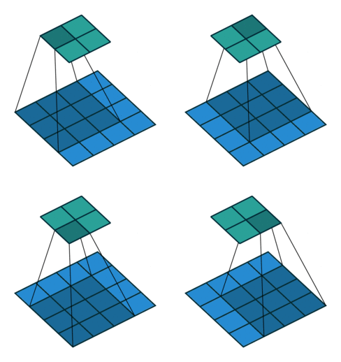
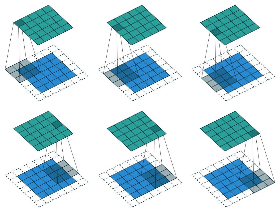
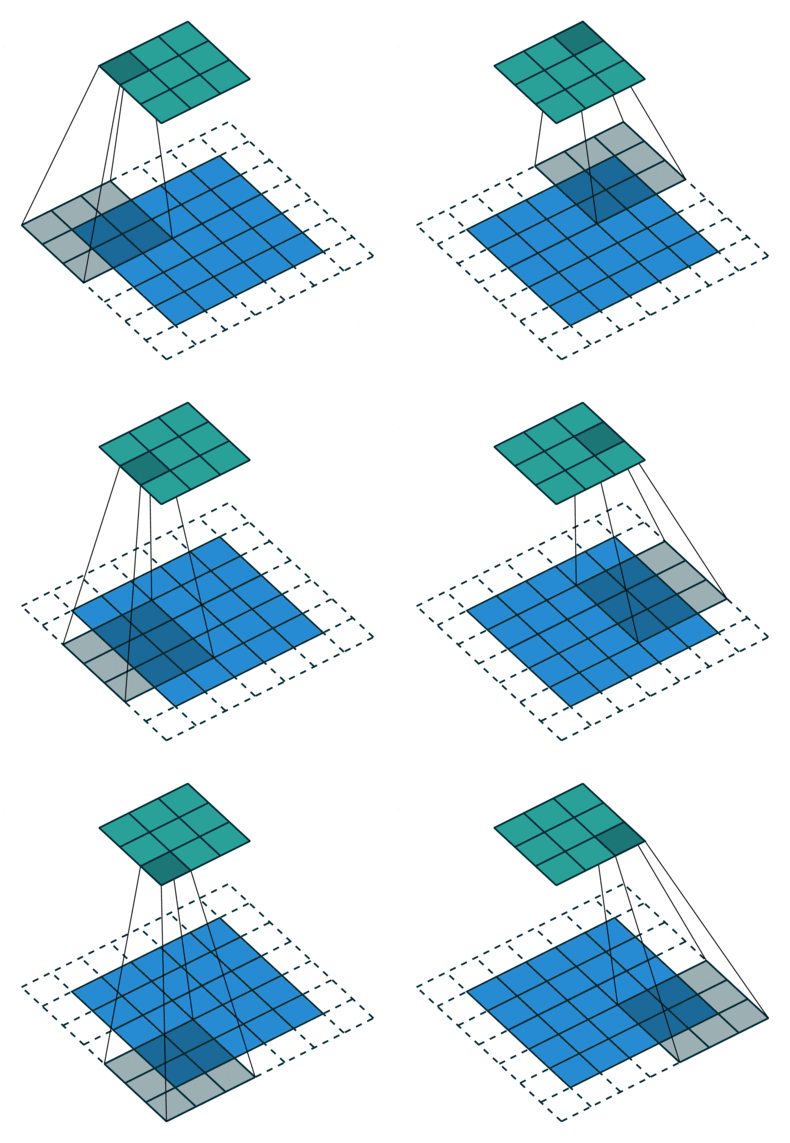
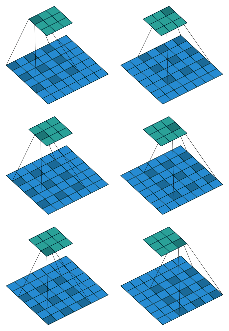
# In the following animations, **blue** maps are inputs,
# **green** maps are outputs and
# the **shaded** area is the kernel with $F=3$.
# 
# | $P=0,~S=1,~D=1$ | $P=1,~S=1,~D=1$ | $P=1,~S=2,~D=1$ | $P=0,~S=1,~D=2$ |
# |-----------------|-----------------|-----------------| --------------- |
# |<img src="https://raw.githubusercontent.com/vdumoulin/conv_arithmetic/master/gif/no_padding_no_strides.gif" width="250"/>| <img src="https://raw.githubusercontent.com/vdumoulin/conv_arithmetic/master/gif/same_padding_no_strides.gif" width="250"/> | <img src="https://raw.githubusercontent.com/vdumoulin/conv_arithmetic/master/gif/padding_strides.gif" width="250"/> | <img src="https://raw.githubusercontent.com/vdumoulin/conv_arithmetic/master/gif/dilation.gif" width="250"/> |
# 
# 
# We can see that the second combination, $F=3,~P=1,~S=1,~D=1$, leads to identical sizes of input and output feature maps.

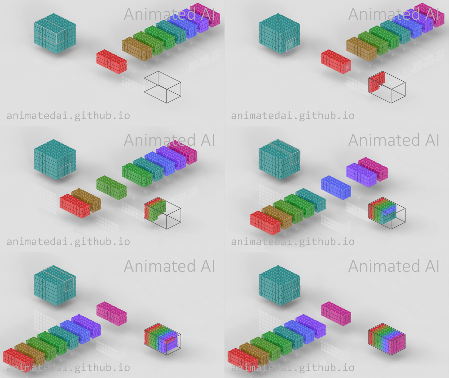
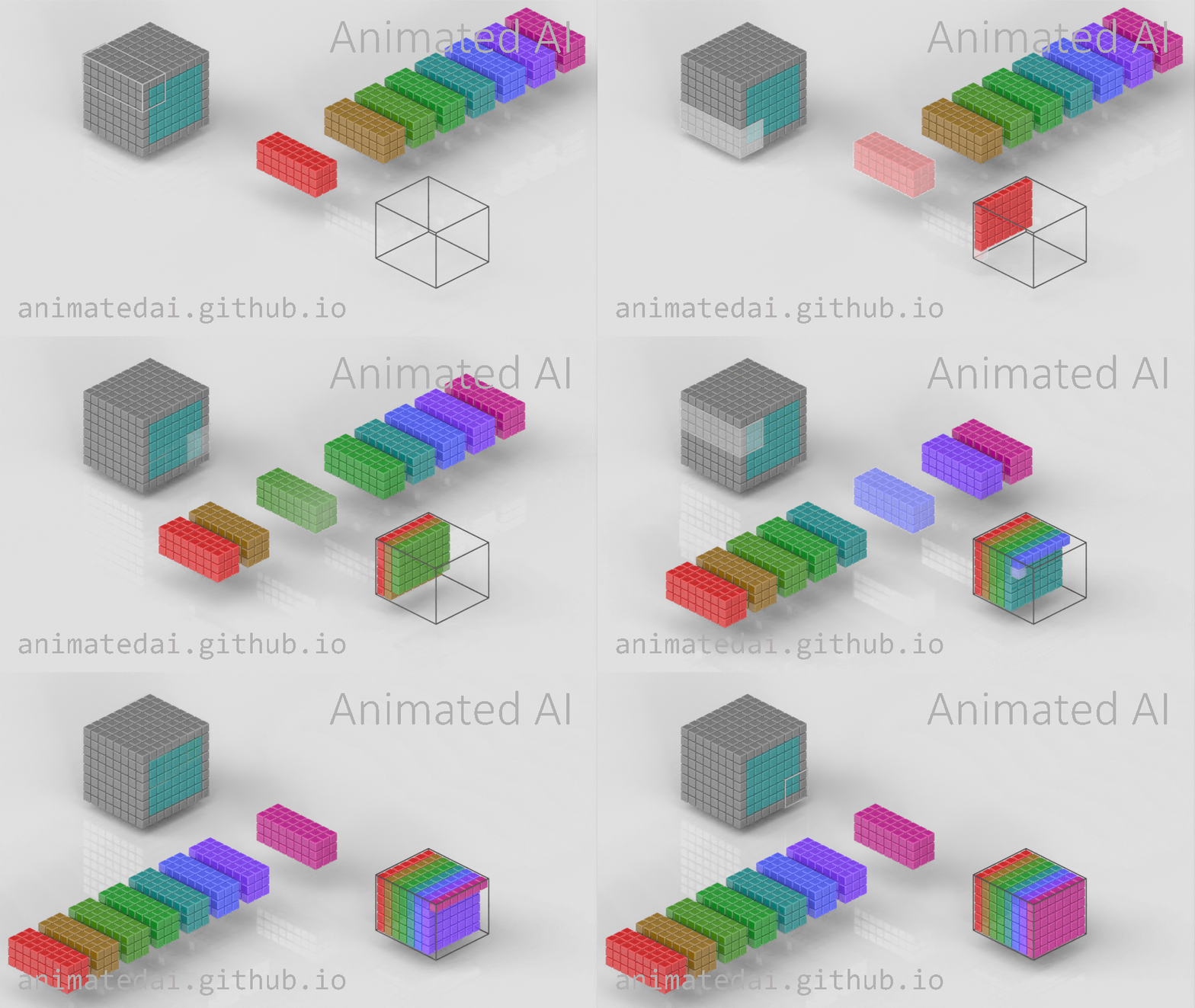
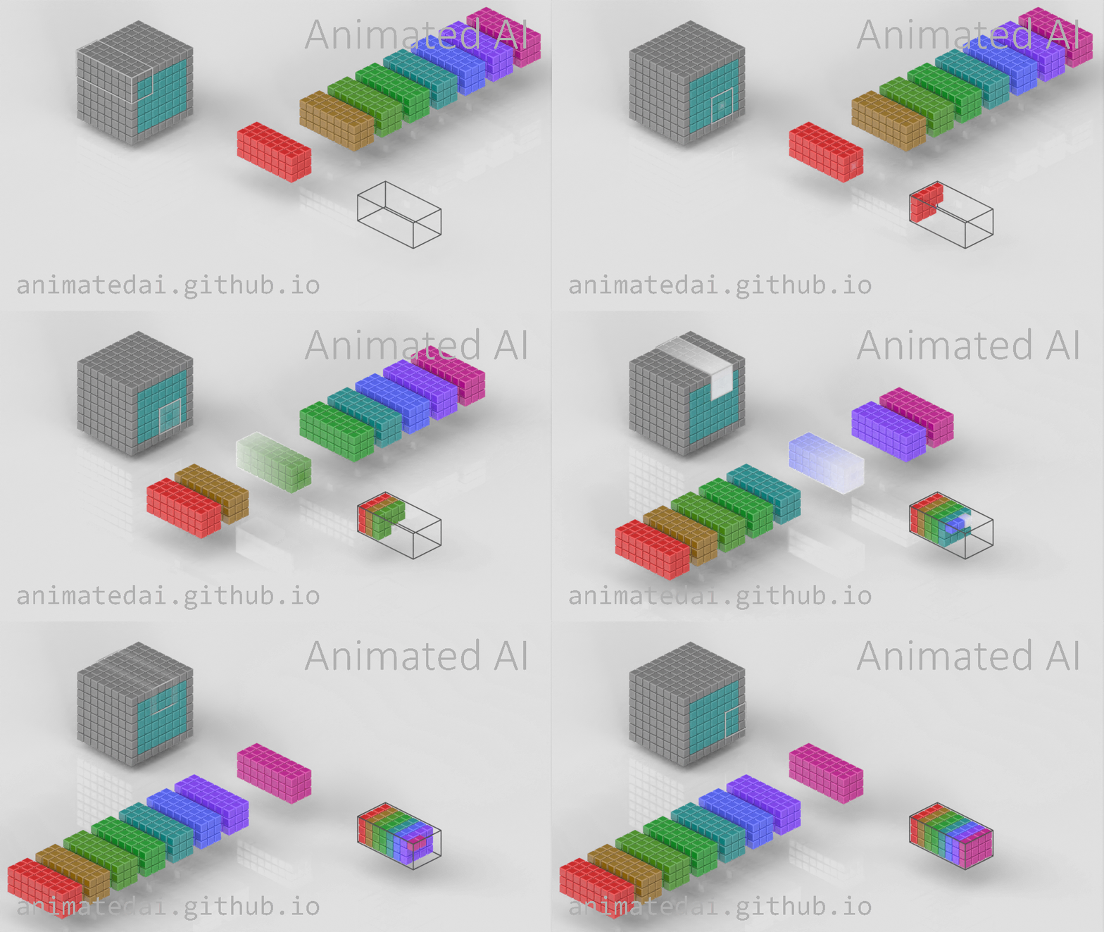
# A 3D view
# 
# | $P=0,~S=1,~D=1$ | $P=1,~S=1,~D=1$ | $P=1,~S=2,~D=1$ |
# |-----------------|-----------------|-----------------|
# |<img src="https://animatedai.github.io/media/convolution-animation-3x3-kernel.gif" width="400"/>| <img src="https://animatedai.github.io/media/convolution-animation-3x3-kernel-same-padding.gif" width="400"/> | <img src="https://animatedai.github.io/media/convolution-animation-3x3-kernel-stride-2-same-padding.gif" width="400"/> | 
# 
# 

# Then, given a set of hyperparameters,
# 
# - Each convolution kernel will (usually) be a tensor of shape $(C_{\mathrm{in}}, F, F)$.
# - The ouput volume dimensions will be:
# 
#   $$\begin{align}
#   H_{\mathrm{out}} &= \left\lfloor \frac{H_{\mathrm{in}} + 2P - D\cdot(F-1) -1}{S} \right\rfloor + 1\\
#   W_{\mathrm{out}} &= \left\lfloor \frac{W_{\mathrm{in}} + 2P - D\cdot(F-1) -1}{S} \right\rfloor + 1\\
#   C_{\mathrm{out}} &= K\\
#   \end{align}$$

# - The number of parameters in a convolutional **layer** will be:

# $$
# \underbrace{K}_{\mathrm{kernels}} \cdot \left(
# \underbrace{C_{\mathrm{in}} \cdot F^2}_{\mathrm{kernel\ parameters}} + \underbrace{1}_{\mathrm{bias\ term}}
# \right)
# $$

# **Example**: Input image is 1000x1000x3, and the first conv layer has $10$ kernels of size 5x5.
# The number of parameters in the first layer will be: $ 10 \cdot 3 \cdot 5^2 + 10 = 760 $.
# 

# ### Pytorch `Conv2d` layer example

# In[3]:


import torchvision.transforms as tvtf

tf = tvtf.Compose([tvtf.ToTensor()])
ds_cifar10 = torchvision.datasets.CIFAR10(data_dir, download=True, train=True, transform=tf)


# In[4]:


# Load first CIFAR10 image
x0,y0 = ds_cifar10[0]

# add batch dimension
x0 = x0.unsqueeze(0)

# Note: channels come before spatial extent
print('x0 shape with batch dim:', x0.shape)


# In[5]:


# A function to count the number of parameters in an nn.Module.
def num_params(layer):
    return sum([p.numel() for p in layer.parameters()])


# Let's create our first conv layer with pytorch:

# In[7]:


import torch.nn as nn

# First conv layer: works on input image volume
conv1 = nn.Conv2d(in_channels=x0.shape[1], out_channels=10, padding=1, kernel_size=5, stride=1,dialation=1)

print(f'conv1: {num_params(conv1)} parameters')


# Number of parameters: $10\cdot(3\cdot3^2+1)=280$

# In[8]:


# Apply the layer to an input
print(f'{"Input image shape:":25s}{x0.shape}')

y1 = conv1(x0)
print(f'{"After first conv layer:":25s}{y1.shape}')


# In[9]:


# Second conv layer: works on output volume of first layer
conv2 = nn.Conv2d(in_channels=10, out_channels=20, padding=0, kernel_size=7, stride=2)
print(f'conv2: {num_params(conv2)} parameters')

y2 = conv2(conv1(x0))
print(f'{"After second conv layer:":25s}{y2.shape}')


# New spatial extent:
# 
# $$
# H_{\mathrm{out}} = \left\lfloor \frac{H_{\mathrm{in}} + 2P -F}{S} \right\rfloor + 1
# =
# \left\lfloor \frac{32 + 2\cdot 0 -6}{2} \right\rfloor + 1
# =
# 14
# $$
# 

# **Note**: observe that the width and height dimensions of the input image were never specified!
# more on the significance of that later.

# ## Pooling layers

# In addition to strides, another way to reduce the size of feature maps between the convolutional layers,
# is by adding **pooling** layers.

# A pooling layer has the following hyperparameters (but **no trainable parameters**):
# 
# 1. Spatial extent (size) of each pooling kernel, $F \geq 2$. 
# 1. Stride $S\geq 2$: spatial distance between consecutive applications.
# 1. Operation (e.g. max, average, $p$-norm)
# 
# **Example**: $\max$-pooling with $F=2,~S=2$ performing a factor-2 downsample:
# 
# <center><img src="img/maxpool.png" width="600" /></center>

# ### Why pool feature maps after convolutions?

# One reason is to more rapidly increase the **receptive field** of each layer.
# 
# <center><img src="img/receptive_field2.png" width="500" /></center>

# - Receptive field size increases more rapidly if we add pooling, strides or dilation.
# - We want successive conv layers to be affected by increasingly larger parts of the input image.
# - This allows us to learn a hierarchy of visual features.
# 
# <center><img src="img/feature_hierarchy.png" width="700" /></center>

# Another reason is to add **invariance** to changes in the input.
# 
# - Pooling within feature maps: introduces invariance to small translations
#   <center><img src="img/maxpool.png" width="600" /></center>

# - Pooling across feature maps: introduces invariance to learned transformations
#   <center><img src="img/pooling_invariance.png" width="600" /></center>

# ### PyTorch `Pool2d` layer example

# In[10]:


pool = nn.MaxPool2d(kernel_size=2, stride=2)

print(f'{"After second conv layer:":25s}{conv2(conv1(x0)).shape}')
print(f'{"After max-pool:":25s}{pool(conv2(conv1(x0))).shape}')


# ## Network Architecture

# The basic way to build an architecture of a deep convolutional neural net, is to repeat groups of **conv-relu** layers, optionally add **pooling** in between and end with an **FC-softmax** combination.
# 
# 
# Why does such a scheme make sense, e.g. for image classification?

# <center><img src="img/arch.png" width="700" /></center>

# In the above image,
# 
# - all the **conv** blocks shown are actually **conv-relu** (or some other nonlinearity).
# - The repeating **conv-conv-...-pool** blocks are learned, non-linear feature extractors: they learn to detect specific features in an image (e.g. lines at different orientations).
# - The pooling controls the receptive field increase, so that more high-level features can be generated by each conv group (e.g. shapes composed from multiple simple lines).
# - The **FC-softmax** at the end is just an MLP that uses the extracted features for classification.
# - Training end-to-end learns the classifier together with the features!

# - The rightmost architecture is called VGG, and used to be a relevant architecture for ImageNet classification.
# - Other types of layers, such as normalization layers are usually also added.

# There are many other things to consider as part of the architecture:
# - Size of conv kernels
# - Number of consecutive convolutions
# - Use of batch normalization to speed up training
# - Dropout for improved generalization
# - Not using FC layers (we'll see later)
# - Skip connections (we'll see later)
# 
# All of these could be hyperparameters to cross-validate over!

# Many different network architectures exist, made famous mainly by repeated improvements on the ImageNet classification challenge since 2012.
# 
# <center><img src="img/net_archs.png" width="1100" /></center>

# Notable ImageNet-winning architectures:
# 
# - AlexNet, 5 layers (2012): Based on LeNet, deeper, with ReLU, trained with GPUs
# - Inception/GoogLeNet, 22 layers (2014): Multiple (small) kernel sizes at same depth
# - ResNet, 152 (!) layers (2015): Skip connections

# ### What filters are deep CNNs learning?

# CNNs capture hierarchical features, with deeper layers capturing higher-level, class-specific features
# (Zeiler & Fergus, 2013).
# 
# <center><img src="img/zf1.png" width="1000"/></center>

# This visualization shows patterns which maximally-activate kernels at various layers of a conv net.

# ### PyTorch network architecture example

# Let's implement **LeNet**, arguably the first successful CNN model for MNIST (LeCun, 1998).
# 
# <center><img src="https://cdn-images-1.medium.com/max/1600/1*1TI1aGBZ4dybR6__DI9dzA.png" width="1100" /></center>

# In[11]:


class LeNet(nn.Module):
    def __init__(self, in_channels=3):
        super().__init__()
        self.feature_extractor = nn.Sequential(
            nn.Conv2d(in_channels, out_channels=6, kernel_size=5),
            nn.ReLU(),
            nn.MaxPool2d(2),
            nn.Conv2d(in_channels=6, out_channels=16, kernel_size=5),
            nn.ReLU(),
            nn.MaxPool2d(2),
        )
        self.classifier = nn.Sequential(
            nn.Linear(16*5*5, 120),  # Why 16*5*5 ?
            nn.ReLU(), 
            nn.Linear(120, 84), # (N, 120) -> (N, 84)
            nn.ReLU(),
            nn.Linear(84, 10)   # (N, 84)  -> (N, 10)
        )
    def forward(self, x):
        features = self.feature_extractor(x)
        features = features.view(features.size(0), -1)
        class_scores = self.classifier(features)
        return class_scores


# In[12]:


net = LeNet()
print(net)


# In[13]:


# Test forward pass
print('x0 shape=', x0.shape, end='\n\n')
print('LeNet(x0)=', net(x0), end='\n\n')
print('shape=', net(x0).shape)


# ### Fully-convolutional Networks
# you can read at home, not for the homework

# Notice how we never actually specified the input image size when implementing the network.
# 
# **Does this mean we can use the network on images of any size**?

# **No**, because of the FC layers at the end.
# 
# Here, let's try:

# In[14]:


large_image = torch.randn(1,3,32*2,32*2)
try:
    net(large_image)
except RuntimeError as e:
    print(e, file=sys.stderr)


# However: Only the FC layers at the end require actual knowledge of exact image sizes.

# We can replace them with... More convolutions, of course

# What would we get from:
# 
# - Kernels of size 1x1?
# - Kernels of size HxW (full spatial extent)?
# 
# 
# <center><img src="img/1x1_conv.png" width="600" /></center>

# Lets create a fully-convolutional LeNet:

# In[15]:


class LeNetFullyConv(LeNet):
    def __init__(self):
        super().__init__()
        # Remember: the last feature map volume has shape (16,5,5) for the original image size
        # Override the classifier with 5x5 then 1x1 convolutions
        # Try to figure out the output shape after each of the following convolutions:
        self.classifier = nn.Sequential(
            nn.Conv2d(in_channels=16, out_channels=120, kernel_size=5), # no padding or strides!
            nn.ReLU(),
            nn.Conv2d(in_channels=120, out_channels=84, kernel_size=1), # 1x1 conv
            nn.ReLU(),
            nn.Conv2d(in_channels=84, out_channels=10, kernel_size=1),  # 1x1 conv
        )
        
    def forward(self, x):
        # Using feature extractor block from the base model
        features = self.feature_extractor(x)
        # note: no need to reshape the features now
        class_scores = self.classifier(features)
        return class_scores


# In[16]:


net_fully_conv = LeNetFullyConv()
print(net_fully_conv)


# Let's forward the original-sized image and the larger image through the network and observe the output shapes:

# In[17]:


print('regular image output shape:', net_fully_conv(x0).shape)
print('large   image output shape:', net_fully_conv(large_image).shape)


# **What's the meaning of the output after conversion to fully convolutional?**

# It's now a **spatial classification map**.
# 
# <center><img src="img/fully_conv.png" width="1000" /></center>
# 

# ## Residual Networks

# <center><img src="img/deeper_meme.jpeg"/></center>
# 
# For image-related tasks it seems that **deeper is better**: learn more complex features.
# 
# How deep can we go? Should more depth always improve results?

# In theory, adding an addition layer should provide **at least** the same accuracy as before.

# Extra layers could always be just identity maps.
# 
# In practice, there are two major problems with adding depth:
# 1. More difficult convergence: vanishing gradients
# 1. More difficult optimization: parameter space increases

# <center><img src="img/resnet_plain_deep_error.png" width="800"/></center>
# 
# I.e., even if the same solution (or better) exists, SGD-based optimization can't find it. **Optimization error** increased with depth.

# ResNets attempt to address these issues by building a network architecture composed of convolutional blocks with added **shortcut-connections**:
# 
# <center><img src="img/resnet_block2.png" width="900"/></center>
# 
# (Left: basic block; right: bottleneck block).
# 
# Here the weight layers are `3x3` or `1x1` convolutions followed by batch-normalization.
# 
# **Why do these shortcut-connections help?**

# These shortcuts create two key advantages:
# - Allow gradients to "flow" freely backwards
# - Each block only learns the "residual mapping", i.e. some delta from the identity map which is easier to optimize.

# Implementation: In the homeworks :)

# #### Thanks!

# **Credits**
# 
# This tutorial was written by [Aviv A. Rosenberg](https://avivr.net) and [Moshe Kimhi](https://mkimhi.github.io/).<br>
# To re-use, please provide attribution and link to the original.
# 
# Some images in this tutorial were taken and/or adapted from the following sources:
# 
# - Sebastian Raschka, https://sebastianraschka.com/
# - Deep Learning, Goodfellow, Bengio and Courville, MIT Press, 2016
# - Fundamentals of Deep Learning, Nikhil Buduma, Oreilly 2017
# - Deep Learning with Python, Francios Chollet, Manning 2018
# - Stanford cs231n course notes by Andrej Karpathy
# - https://github.com/vdumoulin/conv_arithmetic
# - Long, J., Shelhamer, E., & Darrell, T. (2015). Fully convolutional networks for semantic segmentation. In Proceedings of the IEEE conference on computer vision and pattern recognition.
# - Canziani, A., Paszke, A., & Culurciello, E. (2016). An analysis of deep neural network models for practical applications.
# - He, K., Zhang, X., Ren, S., & Sun, J. (2016). Deep residual learning for image recognition. In Proceedings of the IEEE conference on computer vision and pattern recognition.
# - A Comprehensive Introduction to Different Types of Convolutions in Deep Learning, Kulun Bai
# - https://animatedai.github.io/

# In[ ]: