#!/usr/bin/env python
# coding: utf-8
# $$
# \newcommand{\mat}[1]{\boldsymbol {#1}}
# \newcommand{\mattr}[1]{\boldsymbol {#1}^\top}
# \newcommand{\matinv}[1]{\boldsymbol {#1}^{-1}}
# \newcommand{\vec}[1]{\boldsymbol {#1}}
# \newcommand{\vectr}[1]{\boldsymbol {#1}^\top}
# \newcommand{\rvar}[1]{\mathrm {#1}}
# \newcommand{\rvec}[1]{\boldsymbol{\mathrm{#1}}}
# \newcommand{\diag}{\mathop{\mathrm {diag}}}
# \newcommand{\set}[1]{\mathbb {#1}}
# \newcommand{\norm}[1]{\left\lVert#1\right\rVert}
# \newcommand{\pderiv}[2]{\frac{\partial #1}{\partial #2}}
# \newcommand{\bb}[1]{\boldsymbol{#1}}
# $$
#
#
# # CS236781: Deep Learning
# # Tutorial 8: Sequence Models
# ## Introduction
#
# In this tutorial, we will cover:
#
# - What RNNs are and how they work
# - Implementing basic RNNs models
# - Application example: sentiment analysis of movie reviews
# - Bonus: Stock prediction
#
# In[1]:
# Setup
get_ipython().run_line_magic('matplotlib', 'inline')
import os
import sys
import time
import torch
import matplotlib.pyplot as plt
import warnings
warnings.simplefilter("ignore")
# pytorch
import torch
import torch.nn as nn
import torchtext
import torchtext.data as data
import torchtext.datasets as datasets
import torch.nn.functional as f
# In[2]:
plt.rcParams['font.size'] = 20
data_dir = os.path.expanduser('~/.pytorch-datasets')
device = torch.device('cuda' if torch.cuda.is_available() else 'cpu')
# ## Theory Reminders
# Thus far, our models have been composed of fully connected (linear) layers or convolutional layers.
# - Fully connected layers
# - Each layer $l$ operates on the output of the previous layer ($\vec{y}_{l-1}$) and calculates,
# $$
# \vec{y}_l = \varphi\left( \mat{W}_l \vec{y}_{l-1} + \vec{b}_l \right),~
# \mat{W}_l\in\set{R}^{n_{l}\times n_{l-1}},~ \vec{b}_l\in\set{R}^{n_l}.
# $$
# - FC's have completely pre-fixed input and output dimensions.
#
#  # How can we model a dynamical system?
#
  #
#
# E.g., a linear system such as
#
# $$\vec{y}_t = a_0 + a_1 \vec{y}_{t-1}+\dots+a_P \vec{y}_{t-P} + b_0 \vec{x}_t+\dots+b_{t-Q}\vec{x}_{t-Q}$$
#
# Many use cases and examples: signal processing, text translation, sentiment analysis, scene classification in video, etc.
# ## NLP Task summery
#
#
#
#
#
# E.g., a linear system such as
#
# $$\vec{y}_t = a_0 + a_1 \vec{y}_{t-1}+\dots+a_P \vec{y}_{t-P} + b_0 \vec{x}_t+\dots+b_{t-Q}\vec{x}_{t-Q}$$
#
# Many use cases and examples: signal processing, text translation, sentiment analysis, scene classification in video, etc.
# ## NLP Task summery
#
#
#  # #### A quick review of the Naive Bayes (NB) method for text classification:
#
# input vector $\mathbf{x} = \langle x_1, x_2, \ldots, x_m \rangle$ of feature values, and a set of classes $\{ c_1, c_2, \ldots, c_k \}$ the text should be classified as.
#
# We will predict the class $c_i$ that maximizes $Pr(c_i \mid \mathbf{x})$.
#
# By Bayes rule (this is the "Bayes" part in the name "Naive Bayes"),
#
# $$ argmax_i Pr(c_i | x) = argmax_i \frac{Pr(\mathbf{x} | c_i) \cdot Pr(c_i)}{Pr(\mathbf{x})} = argmax_i Pr(\mathbf{x} | c_i) \cdot Pr(c_i) $$
#
# What's naive?
# NB called like that because it used the bayes rule, and because it's navie...assuming I.I.D, i.e:
# $$ Pr(\mathbf{x} | c_i) = \prod_{j=1}^m Pr(x_j | c_i) $$
#
# What is $Pr(x_j | c_i)$ ?
# $$ Pr(x_j | c_i) \approx \frac{\# (x_j, c_i)}{\sum_k \# (x_k, c_i)} $$
#
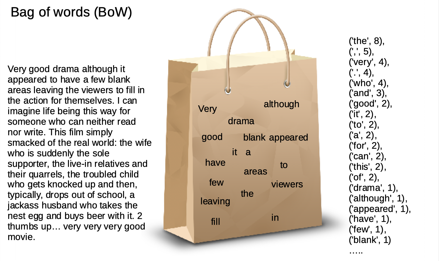
# This counting basic approch. is called **Bag Of Words (BOW)**.
#
# in this approch, we count all the words in the document and use each one as a feature.
# in general, expressing features as raw words is very easy to use with naive base.
#
#  #
# you probably see the problem right away.
#
# you probably see the problem right away.
# The strongest features are now very expresive.. 'the', ',' and 'very' doesn't say much about this review.
#
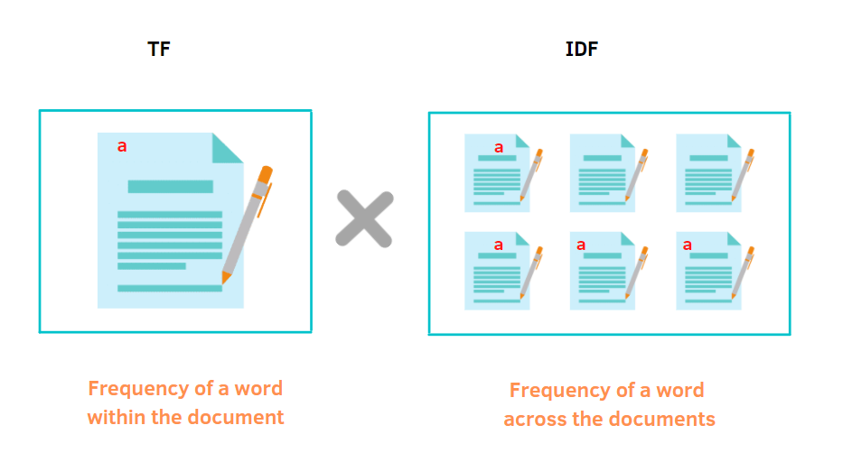
# That's why we need to express, not only the document frequncies, but also the general word frequncies.
# something like that is called **TF-IDF** as **Term frequency–inverse document frequency**
#
#  #
#
# **TF** Like BOW, **IDF** define as $log(\frac{N}{Df_x})$ where N is the num of docs, and Df is the number of documents containing the term x.
#
# $$\# (x_j, c_i) log(\frac{\sum_i \# (c_i)}{\sum_i \# (c_i,x_j)}) $$
#
# and we solved one problem, however, order of words still matter and naive base, ever with smarter representation, is still naive in the notion of corrolation and order.
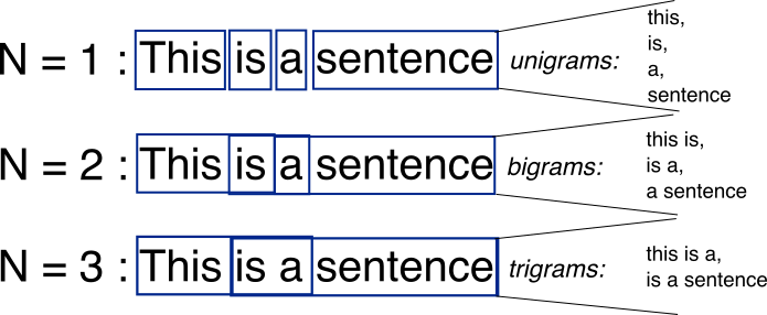
# #### Now text generation, in a nutshell:
#
# A model that predict the next token in a sentence, called **N-gram**.
#
# recall that we have $m$ possible tokens in our corpus, we want to choose the word that maximize:
# $$
# Pr(x_n | x_1, x_2, ..., x_{n-1}) \approx \frac{\#{x_1, x_2, ..., x_n}}{\#{x_1, x_2, ..., x_{n-1}}} = \frac{\#{x_1, x_2, ..., x_n}}{\sum_{x'} \#{x_1, x_2, ..., x_{n-1}, x'}}
# $$
#
# were the lenght of the sequnce that we depand on is the **N**.
#
#
# **TF** Like BOW, **IDF** define as $log(\frac{N}{Df_x})$ where N is the num of docs, and Df is the number of documents containing the term x.
#
# $$\# (x_j, c_i) log(\frac{\sum_i \# (c_i)}{\sum_i \# (c_i,x_j)}) $$
#
# and we solved one problem, however, order of words still matter and naive base, ever with smarter representation, is still naive in the notion of corrolation and order.
# #### Now text generation, in a nutshell:
#
# A model that predict the next token in a sentence, called **N-gram**.
#
# recall that we have $m$ possible tokens in our corpus, we want to choose the word that maximize:
# $$
# Pr(x_n | x_1, x_2, ..., x_{n-1}) \approx \frac{\#{x_1, x_2, ..., x_n}}{\#{x_1, x_2, ..., x_{n-1}}} = \frac{\#{x_1, x_2, ..., x_n}}{\sum_{x'} \#{x_1, x_2, ..., x_{n-1}, x'}}
# $$
#
# were the lenght of the sequnce that we depand on is the **N**.
#
#  #
#
# Now Let's dive into the components that we have in deep learning
# ## Recurrent layers
# An RNN layer is similar to a regular FC layer, but it has two inputs:
# - Current sample, $\vec{x}_t \in\set{R}^{d_{i}}$.
# - Previous **state**, $\vec{h}_{t-1}\in\set{R}^{d_{h}}$.
#
# and it produces two outputs which depend on both:
# - Current layer output, $\vec{y}_t\in\set{R}^{d_o}$.
# - Current **state**, $\vec{h}_{t}\in\set{R}^{d_{h}}$.
#
#
#
# Now Let's dive into the components that we have in deep learning
# ## Recurrent layers
# An RNN layer is similar to a regular FC layer, but it has two inputs:
# - Current sample, $\vec{x}_t \in\set{R}^{d_{i}}$.
# - Previous **state**, $\vec{h}_{t-1}\in\set{R}^{d_{h}}$.
#
# and it produces two outputs which depend on both:
# - Current layer output, $\vec{y}_t\in\set{R}^{d_o}$.
# - Current **state**, $\vec{h}_{t}\in\set{R}^{d_{h}}$.
#  #
# Crucially,
# - The layer itself is not time-dependent (but is parametrized).
# - The same layer (function) is applied at successive time steps, propagating the hidden state.
# A basic RNN can be defined as follows.
#
# $$
# \begin{align}
# \forall t \geq 0:\\
# \vec{h}_t &= \varphi_h\left( \mat{W}_{hh} \vec{h}_{t-1} + \mat{W}_{xh} \vec{x}_t + \vec{b}_h\right) \\
# \vec{y}_t &= \varphi_y\left(\mat{W}_{hy}\vec{h}_t + \vec{b}_y \right)
# \end{align}
# $$
#
# where,
# - $\vec{x}_t \in\set{R}^{d_{i}}$ is the input at time $t$.
# - $\vec{h}_{t-1}\in\set{R}^{d_{h}}$ is the **hidden state** of a fixed dimension.
# - $\vec{y}_t\in\set{R}^{d_o}$ is the output at time $t$.
# - $\mat{W}_{hh}\in\set{R}^{d_h\times d_h}$, $\mat{W}_{xh}\in\set{R}^{d_h\times d_i}$, $\mat{W}_{hy}\in\set{R}^{d_o\times d_h}$, $\vec{b}_h\in\set{R}^{d_h}$ and $\vec{b}_y\in\set{R}^{d_o}$ are the model weights and biases.
# - $\varphi_h$ and $\varphi_y$ are some non-linear functions. In many cases $\varphi_y$ is not used.
# ### Modeling time-dependence
#
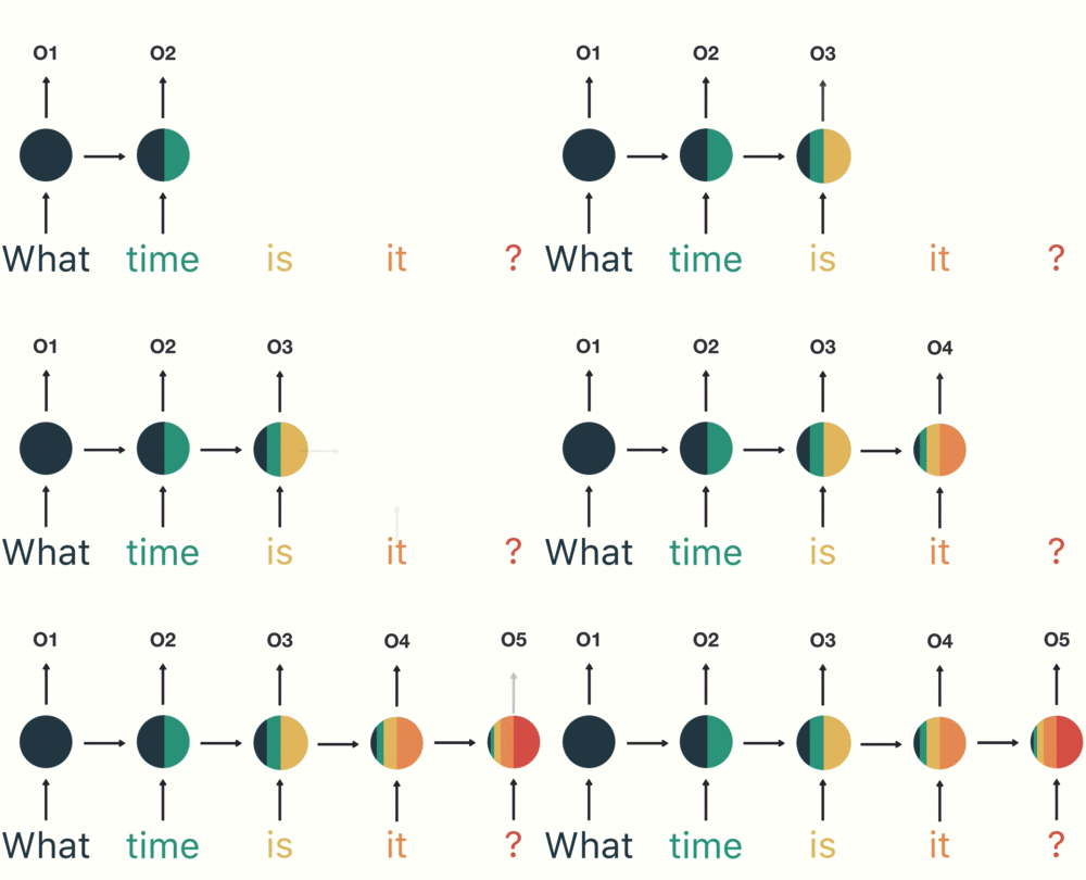
# If we imagine **unrolling** a single RNN layer through time,
#
#
# Crucially,
# - The layer itself is not time-dependent (but is parametrized).
# - The same layer (function) is applied at successive time steps, propagating the hidden state.
# A basic RNN can be defined as follows.
#
# $$
# \begin{align}
# \forall t \geq 0:\\
# \vec{h}_t &= \varphi_h\left( \mat{W}_{hh} \vec{h}_{t-1} + \mat{W}_{xh} \vec{x}_t + \vec{b}_h\right) \\
# \vec{y}_t &= \varphi_y\left(\mat{W}_{hy}\vec{h}_t + \vec{b}_y \right)
# \end{align}
# $$
#
# where,
# - $\vec{x}_t \in\set{R}^{d_{i}}$ is the input at time $t$.
# - $\vec{h}_{t-1}\in\set{R}^{d_{h}}$ is the **hidden state** of a fixed dimension.
# - $\vec{y}_t\in\set{R}^{d_o}$ is the output at time $t$.
# - $\mat{W}_{hh}\in\set{R}^{d_h\times d_h}$, $\mat{W}_{xh}\in\set{R}^{d_h\times d_i}$, $\mat{W}_{hy}\in\set{R}^{d_o\times d_h}$, $\vec{b}_h\in\set{R}^{d_h}$ and $\vec{b}_y\in\set{R}^{d_o}$ are the model weights and biases.
# - $\varphi_h$ and $\varphi_y$ are some non-linear functions. In many cases $\varphi_y$ is not used.
# ### Modeling time-dependence
#
# If we imagine **unrolling** a single RNN layer through time,
#  #
# We can see how late outputs can now be influenced by early inputs, through the hidden state.
# RNN models are very flexible in terms of input and output meaning.
#
# Common applications include image captioning, sentiment analysis, machine translation and signal processing.
#
#
#
# We can see how late outputs can now be influenced by early inputs, through the hidden state.
# RNN models are very flexible in terms of input and output meaning.
#
# Common applications include image captioning, sentiment analysis, machine translation and signal processing.
#
#  #
# How would **backpropagation** work, though?
#
#
# How would **backpropagation** work, though?
#  #
# 1. Calculated loss from each output and accumulate
# 2. Calculate Gradient of loss w.r.t. each parameter at each timestep
# 3. For each parameter, accumulate gradients from all timesteps
# This is known as **Backpropagation through time**, or BPTT.
#
# $$
# \pderiv{L_t}{\mat{W}} = \sum_{k=1}^{t}
# \pderiv{L_t}{\hat y_t} \cdot
# \pderiv{\hat y_t}{\vec{h}_t} \cdot
# \pderiv{\vec{h}_t}{\vec{h}_k} \cdot
# \pderiv{\vec{h}_k}{\mat{W}}
# $$
#
# But how far back do we go? What's the limiting factor?
# We're limited in depth by vanishing and exploding gradients controlled by the eigenvalues of $\mat{W}$.
#
# One pragmatic solution is to limit the number of timesteps involved in the backpropagation.
#
#
#
# 1. Calculated loss from each output and accumulate
# 2. Calculate Gradient of loss w.r.t. each parameter at each timestep
# 3. For each parameter, accumulate gradients from all timesteps
# This is known as **Backpropagation through time**, or BPTT.
#
# $$
# \pderiv{L_t}{\mat{W}} = \sum_{k=1}^{t}
# \pderiv{L_t}{\hat y_t} \cdot
# \pderiv{\hat y_t}{\vec{h}_t} \cdot
# \pderiv{\vec{h}_t}{\vec{h}_k} \cdot
# \pderiv{\vec{h}_k}{\mat{W}}
# $$
#
# But how far back do we go? What's the limiting factor?
# We're limited in depth by vanishing and exploding gradients controlled by the eigenvalues of $\mat{W}$.
#
# One pragmatic solution is to limit the number of timesteps involved in the backpropagation.
#
#  #
# This is known as **Truncated backpropagation through time**, or TBPTT.
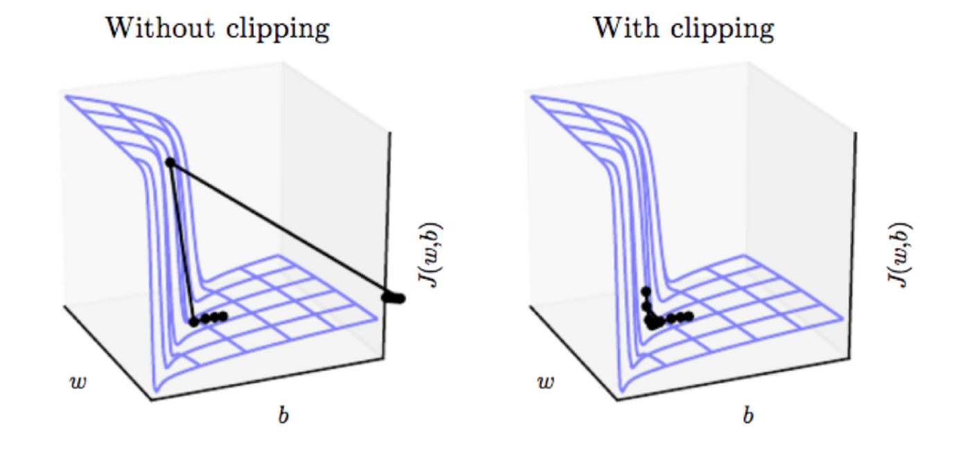
# ### Gradient clipping
# A popular method to avoid exploading gradients, is to use `gradients cliping`
#
# the idea is super simple, yet efficient only for exploading and not for vanishing gradients
#
# the idea is as such:
# look at a layer $\matrix{L}$ with gradient matrix $\matrix{G}$
#
# we would simply look at the norm of the gradients and when they exceed some threshold, we would clip it down.
#
# i.e: if $\norm{\matrix{G}} \ge c$
# $$
# \matrix{G} = C \frac{\matrix{G}}{\norm{\matrix{G}}}
# $$
#
# and the process would look sort of like this:
#
#
# This is known as **Truncated backpropagation through time**, or TBPTT.
# ### Gradient clipping
# A popular method to avoid exploading gradients, is to use `gradients cliping`
#
# the idea is super simple, yet efficient only for exploading and not for vanishing gradients
#
# the idea is as such:
# look at a layer $\matrix{L}$ with gradient matrix $\matrix{G}$
#
# we would simply look at the norm of the gradients and when they exceed some threshold, we would clip it down.
#
# i.e: if $\norm{\matrix{G}} \ge c$
# $$
# \matrix{G} = C \frac{\matrix{G}}{\norm{\matrix{G}}}
# $$
#
# and the process would look sort of like this:
#  # ### Multi-layered (deep) RNN
# RNNs layers can be stacked to build a deep RNN model.
#
#
  #
# - As with MLPs, adding depth allows us to model intricate hierarchical features.
# - However, now we also have a time dimension which makes the representation time-dependent.
# ## RNN Implementation
# Based on the above equations, let's create a simple RNN layer with PyTorch.
# In[3]:
import torch.nn as nn
class RNNLayer(nn.Module):
def __init__(self, in_dim, h_dim, out_dim, phi_h=torch.tanh, phi_y=torch.sigmoid):
super().__init__()
self.phi_h, self.phi_y = phi_h, phi_y
self.fc_xh = nn.Linear(in_dim, h_dim, bias=False)
self.fc_hh = nn.Linear(h_dim, h_dim, bias=True)
self.fc_hy = nn.Linear(h_dim, out_dim, bias=True)
def forward(self, xt, h_prev=None):
if h_prev is None:
h_prev = torch.zeros(xt.shape[0], self.fc_hh.in_features)
ht = self.phi_h(self.fc_xh(xt) + self.fc_hh(h_prev))
yt = self.fc_hy(ht)
if self.phi_y is not None:
yt = self.phi_y(yt)
return yt, ht
# We'll instantiate our model
# In[4]:
N = 3 # batch size
in_dim, h_dim, out_dim = 1024, 10, 1
rnn = RNNLayer(in_dim, h_dim, out_dim)
rnn
# And manually "run" a few time steps
# In[5]:
# t=1
x1 = torch.randn(N, in_dim, requires_grad=True) # requiring grad just for torchviz
y1, h1 = rnn(x1)
print(f'y1 ({tuple(y1.shape)}):\n{y1}')
print(f'h1 ({tuple(h1.shape)}):\n{h1}\n')
# t=2
x2 = torch.randn(N, in_dim, requires_grad=True)
y2, h2 = rnn(x2, h1)
print(f'y2 ({tuple(y2.shape)}):\n{y2}')
print(f'h2 ({tuple(h2.shape)}):\n{h2}\n')
# As usual, let's visualize the computation graph and see what happened when we used the same RNN block twice, by looking at the graph from both $y_1$ and $y_2$.
# In[6]:
import torchviz
torchviz.make_dot(
y2, # Note: Change here to y2 to see the fullly unrolled graph!
params=dict(list(rnn.named_parameters()) + [('x1', x1), ('x2', x2)])
)
# ## LSTM and GRU
#
# We talked about the vanishing gradients problem with RNN, however, we didn't mention how to deal with those.
# Luckyly, Gradient based methods invented long time ago...
# Today we will talk about **Long Short term Memory (LSTM)** and **Gated Recurrent Unit (GRU)**.
#
# both are a type of recurrent cell that tries to preserve long term information. The idea of LSTM was presented back in 1997, but flourished in the age of deep learning.
#
# The cell have `memory` or `context` that's base on the `state` of basic RNN and on 3 main gates:
#
# - Input gate: decides when to read data into the cell.
# - Output gate: outputs the entries from the cell.
# - Forget gate: a mechanism to reset the content of the cell.
#
#
# - The forget gate's output is multiplied with the previous long-term context vector, to decide which old information to exclude.
# - The output gate learns to integrate the current short-term state and input ($O_t$) with the long-term state, to update the short-term hidden state $H_t$.
# - The input gate aggregates the current input $X_t$ and short-term state to update the long-term state.
#
# These gates learn which information is relevant to forget or remember during the training process. The gates contain a non-linear activision function (sigmoid).
# Unlike the RNN, LSTMs maintain two types of hidden states - a short-term hidden state $H_t$, and a long term hidden state, called context, denoted $C_t$.
# The difference in roles is mostly derived from the amount and complexity of computation performed in each cell to compute each.
# * we denote the input $X_t \in \mathbb{R}^{n\times d}$ at timestemp $t$ and the hidden state of the previous time step is $H_{t−1}\in \mathbb{R}^{n\times h}$.
#
#
#
# 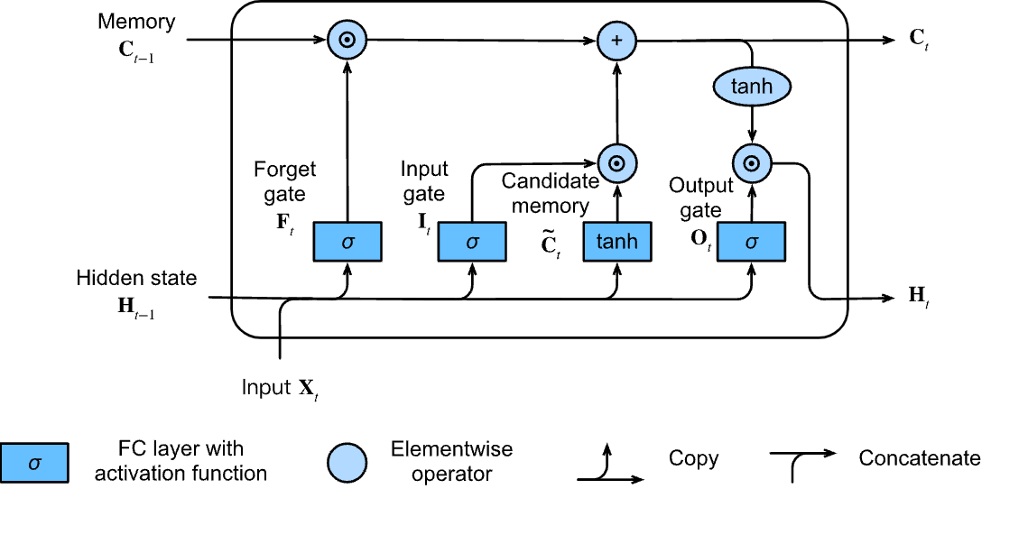 #
# - **Forget gate**: $$ F_t = \sigma(X_tW_{xf} +H_{t-1}W_{hf} +b_f) \in \mathbb{R}^{n\times f}, $$
# - **Input gate**: $$ I_t = \sigma(X_tW_{xi} +H_{t-1}W_{hi} +b_i) \in \mathbb{R}^{n\times h},$$
# - **Output gate**: $$ O_t = \sigma(X_tW_{xo} +H_{t-1}W_{ho} +b_o) \in \mathbb{R}^{n\times o}, $$
#
# - **candidate memory**:$$ \tilde{C}_t = \text{tanh}(X_tW_{xc} +H_{t-1}W_{hc} +b_c) \in \mathbb{R}^{n\times c}$$
#
# - **memory / context**: $$ C_t = F_t \odot C_{t-1} + I_{t} \odot \tilde{C}_t$$
#
# - **hidden state**: $$ H_t = O_t \odot \text{tanh}(C_t)$$
#
#
# as you can see, we save 2 diffrent states, `hidden` and `context` (we have the output as well).
#
# the idea really helps with vanishing gradients, yet a big set of weights is added to the simple RNN.
# In[7]:
lstm = nn.LSTM(10, 20, 2) #LSTM is not an encoder decoder, thus we can project the output size, but default we use the hidden size
input = torch.randn(5, 3, 10) #5 batch size, seq of 3, input dim 10
h0 = torch.randn(2, 3, 20) #2 for 2 layers of the LSTM
c0 = torch.randn(2, 3, 20)
output, (hn, cn) = lstm(input, (h0, c0))
print('input shape =',input.shape)
print('hidden shape =',h0.shape)
print('output shape =',output.shape)
# We now have 8 sets of weights to learn (i.e., the U and W for each of the 4
# gates within each unit), whereas with simple recurrent units we only had 2. Training
# these additional parameters imposes a much significantly higher training cost.
#
# **Gated Recurrent Unit** or **GRU** ease this burden by dispensing with the
# use of a separate context vector, and by reducing the number of gates to 2 — a reset gate, r and an update gate, z.
#
#
#
# - **Forget gate**: $$ F_t = \sigma(X_tW_{xf} +H_{t-1}W_{hf} +b_f) \in \mathbb{R}^{n\times f}, $$
# - **Input gate**: $$ I_t = \sigma(X_tW_{xi} +H_{t-1}W_{hi} +b_i) \in \mathbb{R}^{n\times h},$$
# - **Output gate**: $$ O_t = \sigma(X_tW_{xo} +H_{t-1}W_{ho} +b_o) \in \mathbb{R}^{n\times o}, $$
#
# - **candidate memory**:$$ \tilde{C}_t = \text{tanh}(X_tW_{xc} +H_{t-1}W_{hc} +b_c) \in \mathbb{R}^{n\times c}$$
#
# - **memory / context**: $$ C_t = F_t \odot C_{t-1} + I_{t} \odot \tilde{C}_t$$
#
# - **hidden state**: $$ H_t = O_t \odot \text{tanh}(C_t)$$
#
#
# as you can see, we save 2 diffrent states, `hidden` and `context` (we have the output as well).
#
# the idea really helps with vanishing gradients, yet a big set of weights is added to the simple RNN.
# In[7]:
lstm = nn.LSTM(10, 20, 2) #LSTM is not an encoder decoder, thus we can project the output size, but default we use the hidden size
input = torch.randn(5, 3, 10) #5 batch size, seq of 3, input dim 10
h0 = torch.randn(2, 3, 20) #2 for 2 layers of the LSTM
c0 = torch.randn(2, 3, 20)
output, (hn, cn) = lstm(input, (h0, c0))
print('input shape =',input.shape)
print('hidden shape =',h0.shape)
print('output shape =',output.shape)
# We now have 8 sets of weights to learn (i.e., the U and W for each of the 4
# gates within each unit), whereas with simple recurrent units we only had 2. Training
# these additional parameters imposes a much significantly higher training cost.
#
# **Gated Recurrent Unit** or **GRU** ease this burden by dispensing with the
# use of a separate context vector, and by reducing the number of gates to 2 — a reset gate, r and an update gate, z.
#
#  # - **reset gate**:
# $$ R_t = \sigma(X_tW_{xr} + H_{t-1}W_{hr} +b_r) \in \mathbb{R}^{n \times h}$$
# - **update gate**:
# $$ Z_t = \sigma(X_tW_{xz} + H_{t-1}W_{hz} +b_z) \in \mathbb{R}^{n \times h} $$
#
# - **candidate hidden state**:
# $$ \tilde{H}_{t} = \text{tanh}\left(X_t W_{xh} + (R_t \odot H_{t-1})W_{hh} \right) + b_h$$
# - **hidden state**:
# $$ H_t = Z_t \odot H_{t-1} +(1-Z_t) \odot \tilde{H}_t. $$
#
# * The update gate determines how much the previous hidden state to retain, and how much to get from the new candidate hidden state.
# * The reset gate determines how much of the past information to forget or reset before computing the candidate hidden state.
# * Whenever the update gate $Z_t$ is close to 1, we simply retain the old state. In this case the information from $X_t$ is essentially ignored, effectively skipping time step $t$ in the dependency chain.
# * In contrast, whenever $Z_t$ is close to 0, the new latent state $H_t$ approaches the candidate latent state $\tilde{H}_t$.
# * These designs can help us cope with the vanishing gradient problem in RNNs and better capture dependencies for sequences with large time step distances.
# In[8]:
def num_params(layer):
return sum([p.numel() for p in layer.parameters()])
rnn = nn.RNN(10, 2, 2)
lstm = nn.LSTM(10, 2, 2)
gru = nn.GRU(10,2,2)
print(f'RNN params: {num_params(rnn)}')
print(f'LSTM params: {num_params(lstm)}')
print(f'GRU params: {num_params(gru)}')
# ## Part 1: Sentiment analysis for movie reviews
# The task: Given a review about a movie written by some user, decide whether it's **positive**, **negative** or **neutral**.
#
#
  #
# Classically this is considered a challenging task if approached based on keywords alone.
#
# Consider:
#
# "This movie was actually neither that funny, nor super witty."
#
# To comprehend such a sentence, it's intuitive to see that some "state" must be kept when "reading" it.
# ### Dataset
#
# We'll use the [`torchtext`](https://github.com/pytorch/text) package, which provides useful tools for working ith textual data, and also includes some built-in datasets and dataloaders (similar to `torchvision`).
#
# Out dataset will be the [Stanford Sentiment Treebank](https://nlp.stanford.edu/sentiment/treebank.html) (SST) dataset, which contains ~10,000 **labeled** movie reviews.
#
# The label of each review is either "positive", "neutral" or "negative".
#
# #### Loading and tokenizing text samples
#
# The `torchtext.data.Field` class takes care of splitting text into unique "tokens"
# (~words) and converting it a numerical representation as a sequence of numbers representing
# the tokens in the text.
# In[9]:
#update enviroment locally
#!pip install torchtext==0.6.0
#!pip install nltk
##If you want to run on apple:
#!pip install -U pip setuptools wheel
#!pip install -U 'spacy[apple]'
#!python -m spacy download en_core_web_sm
# In[10]:
import torchtext.data
# torchtext Field objects parse text (e.g. a review) and create a tensor representation
# This Field object will be used for tokenizing the movie reviews text
# For this application, tokens ~= words
review_parser = torchtext.data.Field(
sequential=True, use_vocab=True, lower=True,
init_token='', eos_token='', dtype=torch.long,
tokenize='spacy', tokenizer_language='en_core_web_sm'
)
# This Field object converts the text labels into numeric values (0,1,2)
label_parser = torchtext.data.Field(
is_target=True, sequential=False, unk_token=None, use_vocab=True
)
# In[11]:
import torchtext.datasets
# Load SST, tokenize the samples and labels
# ds_X are Dataset objects which will use the parsers to return tensors
ds_train, ds_valid, ds_test = torchtext.datasets.SST.splits(
review_parser, label_parser, root=data_dir
)
n_train = len(ds_train)
print(f'Number of training samples: {n_train}')
print(f'Number of test samples: {len(ds_test)}')
# Lets print some examples from our training data:
# In[12]:
for i in ([111, 4321, 7777, 0]):
example = ds_train[i]
label = example.label
review = str.join(" ", example.text)
print(f'sample#{i:04d} [{label:8s}]:\n > {review}\n')
# #### Building a vocabulary
#
# The `Field` object can build a **vocabulary** for us,
# which is simply a bi-directional mapping between a unique index and a token.
#
# We'll only include words from the training set in our vocabulary.
# In[13]:
review_parser.build_vocab(ds_train)
label_parser.build_vocab(ds_train)
print(f"Number of tokens in training samples: {len(review_parser.vocab)}")
print(f"Number of tokens in training labels: {len(label_parser.vocab)}")
# In[14]:
print(f'first 20 tokens:\n', review_parser.vocab.itos[:20], end='\n\n')
# Note the **special tokens**, ``, ``, `` and `` at indexes `0-3`.
# These were automatically created by the tokenizer.
# In[15]:
# Show that some words exist in the vocab
for w in ['film', 'actor', 'schwarzenegger', 'spielberg']:
print(f'word={w:15s} index={review_parser.vocab.stoi[w]}')
# In[16]:
print(f'labels vocab:\n', dict(label_parser.vocab.stoi))
# In[17]:
hist = [ds_train[i].label for i in range(len(ds_train))]
plt.hist(hist);
# #### Data loaders (iterators)
#
# The `torchtext` package comes with `Iterator`s, similar to the `DataLoaders` we previously worked with.
#
# A key issue when working with text sequences is that each sample is of a different length.
#
# So, how can we work with **batches** of data?
# In[18]:
BATCH_SIZE = 4
# BucketIterator creates batches with samples of similar length
# to minimize the number of tokens in the batch.
dl_train, dl_valid, dl_test = torchtext.data.BucketIterator.splits(
(ds_train, ds_valid, ds_test), batch_size=BATCH_SIZE,
shuffle=True, device=device)
# Lets look at a single batch.
# In[77]:
batch = next(iter(dl_train))
X, y = batch.text, batch.label
print('X = \n', X, X.shape, end='\n\n')
print('y = \n', y, y.shape)
# What are we looking at?
# Our sample tensor `X` is of shape `(sentence_length, batch_size)`.
#
# Note that:
# 1. `sentence_length` changes every batch! You can re-run the previous block to see this.
# 2. Sequence dimension first (not batch). When we implement the model, you'll see why it's easier to work this way.
# ### Model
#
# We'll now create our sentiment analysis model based on the simple `RNNLayer` we've implemented above.
# The model will:
# - Take an input batch of tokenized sentences.
# - Compute a dense word-embedding of each token.
# - Process the sentence **sequentially** through the RNN layer.
# - Produce a `(B, 3)` tensor, which we'll interpret as class probabilities for each sentence in the batch.
# What is a **word embedding**? How do we get one?
# Embeddings encode tokens as tensors in a way that maintain some **semantic** meaning for our task.
#
#
#
# Classically this is considered a challenging task if approached based on keywords alone.
#
# Consider:
#
# "This movie was actually neither that funny, nor super witty."
#
# To comprehend such a sentence, it's intuitive to see that some "state" must be kept when "reading" it.
# ### Dataset
#
# We'll use the [`torchtext`](https://github.com/pytorch/text) package, which provides useful tools for working ith textual data, and also includes some built-in datasets and dataloaders (similar to `torchvision`).
#
# Out dataset will be the [Stanford Sentiment Treebank](https://nlp.stanford.edu/sentiment/treebank.html) (SST) dataset, which contains ~10,000 **labeled** movie reviews.
#
# The label of each review is either "positive", "neutral" or "negative".
#
# #### Loading and tokenizing text samples
#
# The `torchtext.data.Field` class takes care of splitting text into unique "tokens"
# (~words) and converting it a numerical representation as a sequence of numbers representing
# the tokens in the text.
# In[9]:
#update enviroment locally
#!pip install torchtext==0.6.0
#!pip install nltk
##If you want to run on apple:
#!pip install -U pip setuptools wheel
#!pip install -U 'spacy[apple]'
#!python -m spacy download en_core_web_sm
# In[10]:
import torchtext.data
# torchtext Field objects parse text (e.g. a review) and create a tensor representation
# This Field object will be used for tokenizing the movie reviews text
# For this application, tokens ~= words
review_parser = torchtext.data.Field(
sequential=True, use_vocab=True, lower=True,
init_token='', eos_token='', dtype=torch.long,
tokenize='spacy', tokenizer_language='en_core_web_sm'
)
# This Field object converts the text labels into numeric values (0,1,2)
label_parser = torchtext.data.Field(
is_target=True, sequential=False, unk_token=None, use_vocab=True
)
# In[11]:
import torchtext.datasets
# Load SST, tokenize the samples and labels
# ds_X are Dataset objects which will use the parsers to return tensors
ds_train, ds_valid, ds_test = torchtext.datasets.SST.splits(
review_parser, label_parser, root=data_dir
)
n_train = len(ds_train)
print(f'Number of training samples: {n_train}')
print(f'Number of test samples: {len(ds_test)}')
# Lets print some examples from our training data:
# In[12]:
for i in ([111, 4321, 7777, 0]):
example = ds_train[i]
label = example.label
review = str.join(" ", example.text)
print(f'sample#{i:04d} [{label:8s}]:\n > {review}\n')
# #### Building a vocabulary
#
# The `Field` object can build a **vocabulary** for us,
# which is simply a bi-directional mapping between a unique index and a token.
#
# We'll only include words from the training set in our vocabulary.
# In[13]:
review_parser.build_vocab(ds_train)
label_parser.build_vocab(ds_train)
print(f"Number of tokens in training samples: {len(review_parser.vocab)}")
print(f"Number of tokens in training labels: {len(label_parser.vocab)}")
# In[14]:
print(f'first 20 tokens:\n', review_parser.vocab.itos[:20], end='\n\n')
# Note the **special tokens**, ``, ``, `` and `` at indexes `0-3`.
# These were automatically created by the tokenizer.
# In[15]:
# Show that some words exist in the vocab
for w in ['film', 'actor', 'schwarzenegger', 'spielberg']:
print(f'word={w:15s} index={review_parser.vocab.stoi[w]}')
# In[16]:
print(f'labels vocab:\n', dict(label_parser.vocab.stoi))
# In[17]:
hist = [ds_train[i].label for i in range(len(ds_train))]
plt.hist(hist);
# #### Data loaders (iterators)
#
# The `torchtext` package comes with `Iterator`s, similar to the `DataLoaders` we previously worked with.
#
# A key issue when working with text sequences is that each sample is of a different length.
#
# So, how can we work with **batches** of data?
# In[18]:
BATCH_SIZE = 4
# BucketIterator creates batches with samples of similar length
# to minimize the number of tokens in the batch.
dl_train, dl_valid, dl_test = torchtext.data.BucketIterator.splits(
(ds_train, ds_valid, ds_test), batch_size=BATCH_SIZE,
shuffle=True, device=device)
# Lets look at a single batch.
# In[77]:
batch = next(iter(dl_train))
X, y = batch.text, batch.label
print('X = \n', X, X.shape, end='\n\n')
print('y = \n', y, y.shape)
# What are we looking at?
# Our sample tensor `X` is of shape `(sentence_length, batch_size)`.
#
# Note that:
# 1. `sentence_length` changes every batch! You can re-run the previous block to see this.
# 2. Sequence dimension first (not batch). When we implement the model, you'll see why it's easier to work this way.
# ### Model
#
# We'll now create our sentiment analysis model based on the simple `RNNLayer` we've implemented above.
# The model will:
# - Take an input batch of tokenized sentences.
# - Compute a dense word-embedding of each token.
# - Process the sentence **sequentially** through the RNN layer.
# - Produce a `(B, 3)` tensor, which we'll interpret as class probabilities for each sentence in the batch.
# What is a **word embedding**? How do we get one?
# Embeddings encode tokens as tensors in a way that maintain some **semantic** meaning for our task.
#
#  # ### How we embed:
#
# 1. Embedding Layer: We train an embeding layer with our desired size, take a long time and require a lot of data, but learn the specific relations in our corpus
#
#
# 2. Word2Vec: statistical method for efficiently learning a standalone word embedding from a text corpus. it's based on CBOW (continues bag of words) and C-SKIP-GRAM (continues skip-gram).
#
#
# 3. GloVe (Global Vectors for Word Representation):extension to the word2vec method for efficiently learning word vectors. using matrix factorization techniques such as Latent Semantic Analysis (LSA). if Word2Vec use a window to determine the context, GloVe used the statistics of a word to accure in the global text.
#
#
#
# Here we'll train an Embedding together with our model:
# In[20]:
embedding_layer = nn.Embedding(num_embeddings=5, embedding_dim=8)
token_idx = torch.randint(low=0, high=5, size=(6,))
print(token_idx)
embedding_layer(token_idx)
# OK, model time:
# In[21]:
class SentimentRNN(nn.Module):
def __init__(self, vocab_dim, embedding_dim, h_dim, out_dim):
super().__init__()
# nn.Embedding converts from token index to dense tensor
self.embedding = nn.Embedding(vocab_dim, embedding_dim)
# Our own Vanilla RNN layer, without phi_y so it outputs a class score
self.rnn = RNNLayer(in_dim=embedding_dim, h_dim=h_dim, out_dim=out_dim, phi_y=None)
# To convert class scores to log-probability we'll apply log-softmax
self.log_softmax = nn.LogSoftmax(dim=1)
def forward(self, X):
# X shape: (S, B) Note batch dim is not first!
embedded = self.embedding(X) # embedded shape: (S, B, E)
# Loop over (batch of) tokens in the sentence(s)
ht = None
for xt in embedded: # xt is (B, E)
yt, ht = self.rnn(xt, ht) # yt is (B, D_out)
# Class scores to log-probability
yt_log_proba = self.log_softmax(yt)
return yt_log_proba
# Let's instantiate our model.
# In[22]:
INPUT_DIM = len(review_parser.vocab)
EMBEDDING_DIM = 100
HIDDEN_DIM = 128
OUTPUT_DIM = 3
model = SentimentRNN(INPUT_DIM, EMBEDDING_DIM, HIDDEN_DIM, OUTPUT_DIM)
model
# Test a manual forward pass:
# In[23]:
print(f'model(X) = \n', model(X), model(X).shape)
print(f'labels = ', y)
# How big is our model?
# In[24]:
def count_parameters(model):
return sum(p.numel() for p in model.parameters() if p.requires_grad)
print(f'The RNN model has {count_parameters(model):,} trainable weights.')
# Why so many? We used only one RNN layer.
#
# Where are most of the weights?
# ### Training
#
# Let's complete the example by showing the regular pytorch-style train loop with this model.
#
# We'll run only a few epochs on a small subset just to test that it works.
# In[25]:
def train(model, optimizer, loss_fn, dataloader, max_epochs=100, max_batches=200):
for epoch_idx in range(max_epochs):
total_loss, num_correct = 0, 0
start_time = time.time()
for batch_idx, batch in enumerate(dataloader):
X, y = batch.text, batch.label
# Forward pass
y_pred_log_proba = model(X)
# Backward pass
optimizer.zero_grad()
loss = loss_fn(y_pred_log_proba, y)
loss.backward()
# Weight updates
optimizer.step()
# Calculate accuracy
total_loss += loss.item()
y_pred = torch.argmax(y_pred_log_proba, dim=1)
num_correct += torch.sum(y_pred == y).float().item()
if batch_idx == max_batches-1:
break
print(f"Epoch #{epoch_idx}, loss={total_loss /(max_batches):.3f}, accuracy={num_correct /(max_batches*BATCH_SIZE):.3f}, elapsed={time.time()-start_time:.1f} sec")
# In[26]:
import torch.optim as optim
rnn_model = SentimentRNN(INPUT_DIM, EMBEDDING_DIM, HIDDEN_DIM, OUTPUT_DIM).to(device)
optimizer = optim.Adam(rnn_model.parameters(), lr=1e-3)
# Recall: LogSoftmax + NLL is equiv to CrossEntropy on the class scores
loss_fn = nn.NLLLoss()
train(rnn_model, optimizer, loss_fn, dl_train, max_epochs=4) # just a demo
# In[27]:
from sklearn import metrics
def print_stats(model, dataloader):
model.eval() # put in evaluation mode
trues = []
preds = []
with torch.no_grad():
for data in dataloader:
X, y = data.text.to(device), data.label.to(device)
trues+=list(y.cpu())
y_pred_log_proba = model(X)
predicted = torch.argmax(y_pred_log_proba, dim=1)
preds+= list(predicted.cpu())
print(metrics.classification_report(trues, preds, digits=3))
print_stats(rnn_model, dl_train)
# #### Limitations
#
# As usual this is a very naïve model, just for demonstration.
# It lacks many tricks of the NLP trade, such was pre-trained embeddings,
# gated RNN units, deep or bi-directional models, dropout, etc.
#
# Don't expect SotA results :)
# ## Part 2: Time-Series Forecasting: Predicting Stock Prices Using An LSTM Model
# Now we learned how to work with words and documents, how about making money by forecasting in NASDAQ?
#
# as a disclaimer, i will try to explain, why it's nearly impossible to beat the market, but it's still a great tool to be familiar with, and who knows, maybe you would think out of the box and beat the market, just don't forget to tip your favorit T.A after :)
#
# **this is the oposite of a recomandation to invest with predicting the price of stocks**
# we will run this section regardless on the tutorial, so we're going to import all libraries again...
#
# note that `alpha_vantage` just help us to get the stocks data from https://www.alphavantage.co/.
#
# if you don't want it as part of your enviroment, just use `conda update` with the json file again...
#
# **this is also not a recommandation to use alpha_vantage API, it's you can use yahoo database from pandas or whatever other API, or even scrape the data yourself**
# In[41]:
get_ipython().system(' pip install alpha_vantage -q')
# pip install numpy
import numpy as np
# pip install torch
import torch
import torch.nn as nn
import torch.nn.functional as F
import torch.optim as optim
from torch.utils.data import Dataset
from torch.utils.data import DataLoader
# pip install matplotlib
import matplotlib.pyplot as plt
from matplotlib.pyplot import figure
# pip install alpha_vantage
from alpha_vantage.timeseries import TimeSeries
device = torch.device('cuda' if torch.cuda.is_available() else 'cpu')
# now we need to determine some parameters, and we're going to use a dictionary config for that.
# when usually we deal only with batch size and learning rate, here we devide the keys to some sections (so we actually have a dict of dicts)
# - **alpha_vantage**: what params we want to use (here we use only the closing price and only IBM symbole)
# - **data**: we determine window size, as the input seq len for the model and the split size for train and validation
# - **plots**: just some parameters for the plots
# - **model**: some model params
# - **training**: some parameters for the training process
# In[61]:
config = {
"alpha_vantage": {
"key": 'demo', # Claim your free API key here: https://www.alphavantage.co/support/#api-key
"symbol": "IBM", #can use APPL or anything you would like
"outputsize": "full",
"key_adjusted_close": "5. adjusted close",
},
"data": {
"window_size": 4,
"train_split_size": 0.90,
},
"plots": {
"show_plots": True,
"xticks_interval": 90,
"color_actual": "#001f3f",
"color_train": "#3D9970",
"color_val": "#0074D9",
"color_pred_train": "#3D9970",
"color_pred_val": "#0074D9",
"color_pred_test": "#FF4136",
},
"model": {
"input_size": 1, # since we are only using 1 feature, close price
"num_lstm_layers": 2,
"lstm_size": 32,
"dropout": 0.2,
},
"training": {
"device": "cpu", # "cuda" or "cpu"
"batch_size": 64,
"num_epoch": 100,
"learning_rate": 0.01,
"scheduler_step_size": 40,
}
}
# In[62]:
def download_data(config, plot=True):
# get the data from alpha vantage
ts = TimeSeries(key=config["alpha_vantage"]["key"])
data, meta_data = ts.get_daily_adjusted(config["alpha_vantage"]["symbol"], outputsize=config["alpha_vantage"]["outputsize"])
data_date = [date for date in data.keys()]
data_date.reverse()
data_close_price = [float(data[date][config["alpha_vantage"]["key_adjusted_close"]]) for date in data.keys()]
data_close_price.reverse()
data_close_price = np.array(data_close_price)
num_data_points = len(data_date)
display_date_range = "from " + data_date[0] + " to " + data_date[num_data_points-1]
print("Number data points:", num_data_points, display_date_range)
if plot:
fig = figure(figsize=(25, 5), dpi=80)
fig.patch.set_facecolor((1.0, 1.0, 1.0))
plt.plot(data_date, data_close_price, color=config["plots"]["color_actual"])
xticks = [data_date[i] if ((i%config["plots"]["xticks_interval"]==0 and (num_data_points-i) > config["plots"]["xticks_interval"]) or i==num_data_points-1) else None for i in range(num_data_points)] # make x ticks nice
x = np.arange(0,len(xticks))
plt.xticks(x, xticks, rotation='vertical')
plt.title("Daily close price for " + config["alpha_vantage"]["symbol"] + ", " + display_date_range)
plt.grid(visible=None, axis='y', linestyle='--')
plt.show()
return data_date, data_close_price, num_data_points, display_date_range
data_date, data_close_price, num_data_points, display_date_range = download_data(config)
# In[63]:
class Normalizer():
def __init__(self):
self.mu = None
self.sd = None
def fit_transform(self, x):
self.mu = np.mean(x, axis=(0), keepdims=True)
self.sd = np.std(x, axis=(0), keepdims=True)
normalized_x = (x - self.mu)/self.sd
return normalized_x
def inverse_transform(self, x):
return (x*self.sd) + self.mu
# normalize
scaler = Normalizer()
normalized_data_close_price = scaler.fit_transform(data_close_price)
# In[64]:
def prepare_data_x(x, window_size):
# perform windowing
n_row = x.shape[0] - window_size + 1
output = np.lib.stride_tricks.as_strided(x, shape=(n_row,window_size), strides=(x.strides[0],x.strides[0]))
return output[:-1], output[-1]
def prepare_data_y(x, window_size):
# # perform simple moving average
# output = np.convolve(x, np.ones(window_size), 'valid') / window_size
#even easier, use the next day as label
output = x[window_size:]
return output
def prepare_data(normalized_data_close_price, config, plot=False):
data_x, data_x_unseen = prepare_data_x(normalized_data_close_price, window_size=config["data"]["window_size"])
data_y = prepare_data_y(normalized_data_close_price, window_size=config["data"]["window_size"])
# split dataset
split_index = int(data_y.shape[0]*config["data"]["train_split_size"])
data_x_train = data_x[:split_index]
data_x_val = data_x[split_index:]
data_y_train = data_y[:split_index]
data_y_val = data_y[split_index:]
if plot:
# prepare data for plotting
to_plot_data_y_train = np.zeros(num_data_points)
to_plot_data_y_val = np.zeros(num_data_points)
to_plot_data_y_train[config["data"]["window_size"]:split_index+config["data"]["window_size"]] = scaler.inverse_transform(data_y_train)
to_plot_data_y_val[split_index+config["data"]["window_size"]:] = scaler.inverse_transform(data_y_val)
to_plot_data_y_train = np.where(to_plot_data_y_train == 0, None, to_plot_data_y_train)
to_plot_data_y_val = np.where(to_plot_data_y_val == 0, None, to_plot_data_y_val)
## plots
fig = figure(figsize=(25, 5), dpi=80)
fig.patch.set_facecolor((1.0, 1.0, 1.0))
plt.plot(data_date, to_plot_data_y_train, label="Prices (train)", color=config["plots"]["color_train"])
plt.plot(data_date, to_plot_data_y_val, label="Prices (validation)", color=config["plots"]["color_val"])
xticks = [data_date[i] if ((i%config["plots"]["xticks_interval"]==0 and (num_data_points-i) > config["plots"]["xticks_interval"]) or i==num_data_points-1) else None for i in range(num_data_points)] # make x ticks nice
x = np.arange(0,len(xticks))
plt.xticks(x, xticks, rotation='vertical')
plt.title("Daily close prices for " + config["alpha_vantage"]["symbol"] + " - showing training and validation data")
plt.grid(b=None, which='major', axis='y', linestyle='--')
plt.legend()
plt.show()
return split_index, data_x_train, data_y_train, data_x_val, data_y_val, data_x_unseen
split_index, data_x_train, data_y_train, data_x_val, data_y_val, data_x_unseen = prepare_data(normalized_data_close_price, config)
# In[65]:
class TimeSeriesDataset(Dataset):
def __init__(self, x, y):
x = np.expand_dims(x, 2) # in our case, we have only 1 feature, so we need to convert `x` into [batch, sequence, features] for the model
self.x = x.astype(np.float32)
self.y = y.astype(np.float32)
def __len__(self):
return len(self.x)
def __getitem__(self, idx):
return (self.x[idx], self.y[idx])
dataset_train = TimeSeriesDataset(data_x_train, data_y_train)
dataset_val = TimeSeriesDataset(data_x_val, data_y_val)
print("Train data shape", dataset_train.x.shape, dataset_train.y.shape)
print("Validation data shape", dataset_val.x.shape, dataset_val.y.shape)
# In[66]:
class GRU_stocks_Model(nn.Module):
def __init__(self, input_size=1, hidden_layer_size=32, num_layers=2, output_size=1, dropout=0.2):
super().__init__()
self.hidden_layer_size = hidden_layer_size
self.linear_1 = nn.Linear(input_size, hidden_layer_size)
self.relu = nn.ReLU()
self.gru = nn.GRU(hidden_layer_size, hidden_size=self.hidden_layer_size, num_layers=num_layers, batch_first=True)
self.dropout = nn.Dropout(dropout)
self.linear_2 = nn.Linear(num_layers*hidden_layer_size, output_size)
self.init_weights()
def init_weights(self):
for name, param in self.gru.named_parameters():
if 'bias' in name:
nn.init.constant_(param, 0.0)
elif 'weight_ih' in name:
nn.init.kaiming_normal_(param)
elif 'weight_hh' in name:
nn.init.orthogonal_(param)
def forward(self, x):
batchsize = x.shape[0]
# layer 1
x = self.linear_1(x)
x = self.relu(x)
#gru
#if you choose to use lstm:
#lstm_out, (h_n, c_n) = self.lstm(x)
gru_out, h_n = self.gru(x)
# reshape output from hidden cell into [batch, features] for `linear_2`
x = h_n.permute(1, 0, 2).reshape(batchsize, -1)
# layer 2
x = self.dropout(x)
predictions = self.linear_2(x)
return predictions[:,-1]
stocks_Model = GRU_stocks_Model(input_size=config["model"]["input_size"], hidden_layer_size=config["model"]["lstm_size"], num_layers=config["model"]["num_lstm_layers"], output_size=1, dropout=config["model"]["dropout"])
stocks_Model = stocks_Model.to(config["training"]["device"])
# In[67]:
def run_epoch(dataloader, is_training=False):
epoch_loss = 0
if is_training:
stocks_Model.train()
else:
stocks_Model.eval()
for idx, (x, y) in enumerate(dataloader):
if is_training:
optimizer.zero_grad()
batchsize = x.shape[0]
x = x.to(config["training"]["device"])
y = y.to(config["training"]["device"])
out = stocks_Model(x)
loss = criterion(out.contiguous(), y.contiguous())
if is_training:
loss.backward()
optimizer.step()
epoch_loss += (loss.detach().item() / batchsize)
lr = scheduler.get_last_lr()[0]
return epoch_loss, lr
# create `DataLoader`
train_dataloader = DataLoader(dataset_train, batch_size=config["training"]["batch_size"], shuffle=True)
val_dataloader = DataLoader(dataset_val, batch_size=config["training"]["batch_size"], shuffle=True)
# define optimizer, scheduler and loss function
criterion = nn.MSELoss()
optimizer = optim.Adam(stocks_Model.parameters(), lr=config["training"]["learning_rate"], betas=(0.9, 0.98), eps=1e-9)
scheduler = optim.lr_scheduler.StepLR(optimizer, step_size=config["training"]["scheduler_step_size"], gamma=0.1)
# begin training
for epoch in range(config["training"]["num_epoch"]):
loss_train, lr_train = run_epoch(train_dataloader, is_training=True)
loss_val, lr_val = run_epoch(val_dataloader)
scheduler.step()
if epoch%10 ==0:
print('Epoch[{}/{}] | loss train:{:.6f}, test:{:.6f} | lr:{:.6f}'
.format(epoch+1, config["training"]["num_epoch"], loss_train, loss_val, lr_train))
# In[70]:
# here we re-initialize dataloader so the data doesn't shuffled, so we can plot the values by date
train_dataloader = DataLoader(dataset_train, batch_size=config["training"]["batch_size"], shuffle=False)
val_dataloader = DataLoader(dataset_val, batch_size=config["training"]["batch_size"], shuffle=False)
stocks_Model.eval()
# predict on the training data, to see how well the model managed to learn and memorize
predicted_train = np.array([])
for idx, (x, y) in enumerate(train_dataloader):
x = x.to(config["training"]["device"])
out = stocks_Model(x)
out = out.cpu().detach().numpy()
predicted_train = np.concatenate((predicted_train, out))
# predict on the validation data, to see how the model does
predicted_val = np.array([])
for idx, (x, y) in enumerate(val_dataloader):
x = x.to(config["training"]["device"])
out = stocks_Model(x)
out = out.cpu().detach().numpy()
predicted_val = np.concatenate((predicted_val, out))
if config["plots"]["show_plots"]:
# prepare data for plotting, show predicted prices
to_plot_data_y_train_pred = np.zeros(num_data_points)
to_plot_data_y_val_pred = np.zeros(num_data_points)
to_plot_data_y_train_pred[config["data"]["window_size"]:split_index+config["data"]["window_size"]] = scaler.inverse_transform(predicted_train)
to_plot_data_y_val_pred[split_index+config["data"]["window_size"]:] = scaler.inverse_transform(predicted_val)
to_plot_data_y_train_pred = np.where(to_plot_data_y_train_pred == 0, None, to_plot_data_y_train_pred)
to_plot_data_y_val_pred = np.where(to_plot_data_y_val_pred == 0, None, to_plot_data_y_val_pred)
# plots
fig = figure(figsize=(25, 5), dpi=80)
fig.patch.set_facecolor((1.0, 1.0, 1.0))
plt.plot(data_date, data_close_price, label="Actual prices", color=config["plots"]["color_actual"])
plt.plot(data_date, to_plot_data_y_train_pred, label="Predicted prices (train)", color=config["plots"]["color_pred_train"])
plt.plot(data_date, to_plot_data_y_val_pred, label="Predicted prices (validation)", color=config["plots"]["color_pred_val"])
plt.title("Compare predicted prices to actual prices")
xticks = [data_date[i] if ((i%config["plots"]["xticks_interval"]==0 and (num_data_points-i) > config["plots"]["xticks_interval"]) or i==num_data_points-1) else None for i in range(num_data_points)] # make x ticks nice
x = np.arange(0,len(xticks))
plt.xticks(x, xticks, rotation='vertical')
plt.grid(visible=None, which='major', axis='y', linestyle='--')
plt.legend()
plt.show()
# prepare data for plotting, zoom in validation
to_plot_data_y_val_subset = scaler.inverse_transform(data_y_val)
to_plot_predicted_val = scaler.inverse_transform(predicted_val)
to_plot_data_date = data_date[split_index+config["data"]["window_size"]:]
# plots
fig = figure(figsize=(25, 5), dpi=80)
fig.patch.set_facecolor((1.0, 1.0, 1.0))
plt.plot(to_plot_data_date, to_plot_data_y_val_subset, label="Actual prices", color=config["plots"]["color_actual"])
plt.plot(to_plot_data_date, to_plot_predicted_val, label="Predicted prices (validation)", color=config["plots"]["color_pred_val"])
plt.title("Zoom in to examine predicted price on validation data portion")
xticks = [to_plot_data_date[i] if ((i%int(config["plots"]["xticks_interval"]/5)==0 and (len(to_plot_data_date)-i) > config["plots"]["xticks_interval"]/6) or i==len(to_plot_data_date)-1) else None for i in range(len(to_plot_data_date))] # make x ticks nice
xs = np.arange(0,len(xticks))
plt.xticks(xs, xticks, rotation='vertical')
plt.grid(visible=None, which='major', axis='y', linestyle='--')
plt.legend()
plt.show()
# In[72]:
# predict on the unseen data, tomorrow's price
stocks_Model.eval()
x = torch.tensor(data_x_unseen).float().to(config["training"]["device"]).unsqueeze(0).unsqueeze(2) # this is the data type and shape required, [batch, sequence, feature]
prediction = stocks_Model(x)
prediction = prediction.cpu().detach().numpy()
prediction = scaler.inverse_transform(prediction)[0]
if config["plots"]["show_plots"]:
# prepare plots
plot_range = 10
to_plot_data_y_val = np.zeros(plot_range)
to_plot_data_y_val_pred = np.zeros(plot_range)
to_plot_data_y_test_pred = np.zeros(plot_range)
to_plot_data_y_val[:plot_range-1] = scaler.inverse_transform(data_y_val)[-plot_range+1:]
to_plot_data_y_val_pred[:plot_range-1] = scaler.inverse_transform(predicted_val)[-plot_range+1:]
to_plot_data_y_test_pred[plot_range-1] = prediction
to_plot_data_y_val = np.where(to_plot_data_y_val == 0, None, to_plot_data_y_val)
to_plot_data_y_val_pred = np.where(to_plot_data_y_val_pred == 0, None, to_plot_data_y_val_pred)
to_plot_data_y_test_pred = np.where(to_plot_data_y_test_pred == 0, None, to_plot_data_y_test_pred)
# plot
plot_date_test = data_date[-plot_range+1:]
plot_date_test.append("next trading day")
fig = figure(figsize=(25, 5), dpi=80)
fig.patch.set_facecolor((1.0, 1.0, 1.0))
plt.plot(plot_date_test, to_plot_data_y_val, label="Actual prices", marker=".", markersize=10, color=config["plots"]["color_actual"])
plt.plot(plot_date_test, to_plot_data_y_val_pred, label="Past predicted prices", marker=".", markersize=10, color=config["plots"]["color_pred_val"])
plt.plot(plot_date_test, to_plot_data_y_test_pred, label="Predicted price for next day", marker=".", markersize=20, color=config["plots"]["color_pred_test"])
plt.title("Predicted close price of the next trading day")
plt.grid(visible=None, which='major', axis='y', linestyle='--')
plt.legend()
plt.show()
print("Predicted close price of the next trading day:", round(prediction, 2))
# #### Thanks!
# **Credits**
#
# This tutorial was written by [Moshe Kimhi](https://mkimhi.github.io/) and [Aviv A. Rosenberg](https://avivr.net).
# To re-use, please provide attribution and link to the original.
#
# Some images in this tutorial were taken and/or adapted from the following sources:
#
# - Fundamentals of Deep Learning, Nikhil Buduma, Oreilly 2017
# - Sebastian Ruder, "On word embeddings - Part 1", 2016, https://ruder.io
# - Andrej Karpathy, http://karpathy.github.io
# - MIT 6.S191
# - Stanford cs231n
# - S. Bai et al. 2018, http://arxiv.org/abs/1803.01271
# In[ ]:


