#!/usr/bin/env python
# coding: utf-8
# # Linear algebra (review)
# * Linear systems of equations arise widely in numerical methods:
# * nonlinear equations
# * ODEs
# * PDEs
# * interpolation
# * integration
# * quadrature
# * etc.
# * Facility with, and understanding of linear systems, and their geometric interpretations is important.
# * See this [collection of videos](https://www.youtube.com/playlist?list=PLZHQObOWTQDPD3MizzM2xVFitgF8hE_ab).
#
#
#
# ### Linear systems
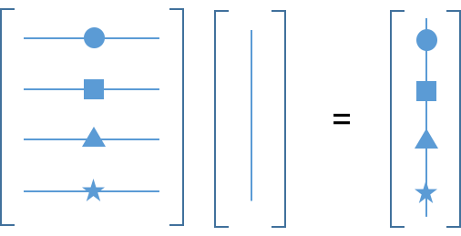
# * Write as $Ax = b$, where $A$ is a matrix and $x$, $b$ are vectors.
# * A is an $m \times n$ matrix: $m$ rows and $n$ columns. Usually, $m=n$
#
#
#
# ### Matrix multiplication
# $b_i = \sum_j a_{i,j}x_j$
#
# **2 interpretations**
#
# (1) A acts on x to produce b
#  #
# (2) x acts on A to produce b
#
#
# (2) x acts on A to produce b
# 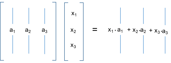 #
# * $b$ is a linear combination of columns of $A$
# * Coordinates of vector $x$ define scalar multipliers in the combination of the columns of $A$.
# * Columns of $A$ are vectors: we combine them through $x$ to get a new vector $b$.
# * Elements of $x$ are like coordinates in the columns of $A$, instead of our usual $\vec{i}$, $\vec{j}$, $\vec{k}$ vector coordinates.
#
# For matrix-matrix multiplication, this process is repeated:
#
#
# * $b$ is a linear combination of columns of $A$
# * Coordinates of vector $x$ define scalar multipliers in the combination of the columns of $A$.
# * Columns of $A$ are vectors: we combine them through $x$ to get a new vector $b$.
# * Elements of $x$ are like coordinates in the columns of $A$, instead of our usual $\vec{i}$, $\vec{j}$, $\vec{k}$ vector coordinates.
#
# For matrix-matrix multiplication, this process is repeated:
#  # * Here, the columns of $C$ are linear combinations of the columns of $A$, where elements of $B$ are the multipliers in those linear combinations.
#
# Also:
#
# * Here, the columns of $C$ are linear combinations of the columns of $A$, where elements of $B$ are the multipliers in those linear combinations.
#
# Also:
# 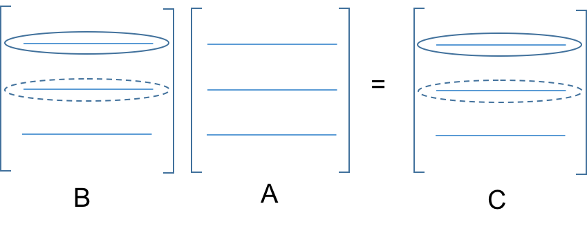 # * Here, the rows of $C$ are linear combinations of the rows of $A$, where elements of $B$ are the multipliers in those linear combinations.
#
# **Identities:**
# * $(AB)^T = B^TA^T$
# * $(AB)^{-1} = B^{-1}A^{-1}$
# ### Definitions
#
# * **Range:** the set of vectors (b) that can be written as $Ax=b$ for some $x$. This is the space spanned by the columns of $A$ since $b$ is a linear combination of the columns of $A$.
# * **Rank:** the number of linearly independent rows or columns.
# * for $m\times n$ with full rank with $m\le n \rightarrow$ rank is $m$.
# * **Basis:** a basis of vectors spans the space and is linearly independent.
# * **Inner product:** $x^Tx \rightarrow s$ where $s$ is a scalar.
# * **Outer product:** $xx^T \rightarrow M$ where $M$ is a matrix. (What's the rank?)
# * **Nonsingular** matrices are invertable and have solutions to $Ax=b$.
#
# Consider 2D plane:
#
# * Here, the rows of $C$ are linear combinations of the rows of $A$, where elements of $B$ are the multipliers in those linear combinations.
#
# **Identities:**
# * $(AB)^T = B^TA^T$
# * $(AB)^{-1} = B^{-1}A^{-1}$
# ### Definitions
#
# * **Range:** the set of vectors (b) that can be written as $Ax=b$ for some $x$. This is the space spanned by the columns of $A$ since $b$ is a linear combination of the columns of $A$.
# * **Rank:** the number of linearly independent rows or columns.
# * for $m\times n$ with full rank with $m\le n \rightarrow$ rank is $m$.
# * **Basis:** a basis of vectors spans the space and is linearly independent.
# * **Inner product:** $x^Tx \rightarrow s$ where $s$ is a scalar.
# * **Outer product:** $xx^T \rightarrow M$ where $M$ is a matrix. (What's the rank?)
# * **Nonsingular** matrices are invertable and have solutions to $Ax=b$.
#
# Consider 2D plane:
# 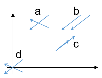 #
# * Case a is a unique solution.
# * Case b has no solution.
# * Case c has $\infty$ solutions
# * Case d is a trivial solution
#
# Numerically singular matrices are *almost* singular. That is, they may be singular to within roundoff error, or the near singularity may result in inaccurate results.
#
# ### Basis, coordinate systems
# $Ax=b$
#
# $x=A^{-1}b$.
#
# * Think of $A$ in terms of its column vectors:
#
#
# * Case a is a unique solution.
# * Case b has no solution.
# * Case c has $\infty$ solutions
# * Case d is a trivial solution
#
# Numerically singular matrices are *almost* singular. That is, they may be singular to within roundoff error, or the near singularity may result in inaccurate results.
#
# ### Basis, coordinate systems
# $Ax=b$
#
# $x=A^{-1}b$.
#
# * Think of $A$ in terms of its column vectors:
# 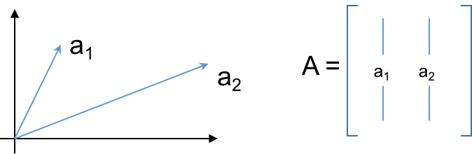 # * For $A\cdot x$, $x$ are the coordinates in the basis of columns of $A$: $a_1$ and $a_2$.
# * For given $b$, $x$ is the vector of coefficients of the unique linear expansion of b in the basis of columns of $A$.
# * **x is b in basis of A**
# * $x$ are coefficients of $b$ in the columns of $A$.
# * $b$ are the coefficients of $b$ in the columns of $I$.
#
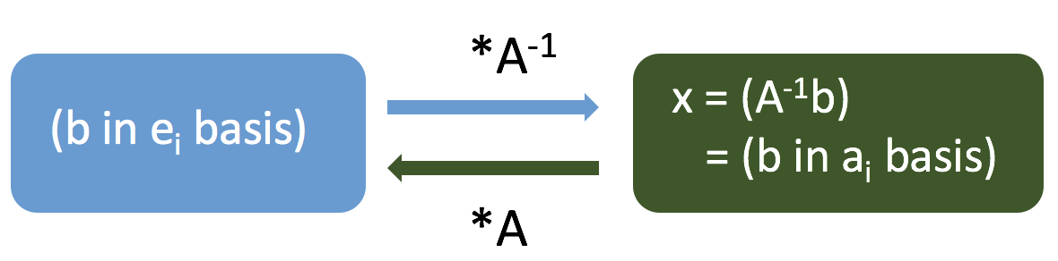
# $A^{-1}b \rightarrow$ **change basis** of $b$:
# * Normally, when we write $x^T = (x_1, x_2)$, we mean $x = x_1\vec{i} + x_2\vec{j}$, or $x = x_1\cdot(1,0)+x_2\cdot(0,1)$.
# * Let $e_i$ be the coordinate vectors, so $e_1 = \vec{i}$ and $e_2 = \vec{j}$, etc.
#
# * For $A\cdot x$, $x$ are the coordinates in the basis of columns of $A$: $a_1$ and $a_2$.
# * For given $b$, $x$ is the vector of coefficients of the unique linear expansion of b in the basis of columns of $A$.
# * **x is b in basis of A**
# * $x$ are coefficients of $b$ in the columns of $A$.
# * $b$ are the coefficients of $b$ in the columns of $I$.
#
# $A^{-1}b \rightarrow$ **change basis** of $b$:
# * Normally, when we write $x^T = (x_1, x_2)$, we mean $x = x_1\vec{i} + x_2\vec{j}$, or $x = x_1\cdot(1,0)+x_2\cdot(0,1)$.
# * Let $e_i$ be the coordinate vectors, so $e_1 = \vec{i}$ and $e_2 = \vec{j}$, etc.
#  # In[10]:
import numpy as np
import matplotlib.pyplot as plt
import matplotlib.cm as cm
get_ipython().run_line_magic('matplotlib', 'inline')
A = np.array([[1, 2],[0, 1]])
n=21
colors = cm.viridis(np.linspace(0, 1, n))
θ = np.linspace(0,2*np.pi,n)
x_0 = np.cos(θ)
x_1 = np.sin(θ)
ϕ_0 = np.zeros(len(x_0))
ϕ_1 = np.zeros(len(x_1))
for i in range(len(x_0)):
x = np.array([x_0[i], x_1[i]])
ϕ = A.dot(x)
ϕ_0[i] = ϕ[0]
ϕ_1[i] = ϕ[1]
#------------------- plot result
plt.figure(figsize=(5,5))
plt.rc('font', size=14)
plt.plot(x_0,x_1, '-', color='gray', label='x') # x
plt.scatter(x_0,x_1, color=colors, s=50, label='') # x
plt.plot(ϕ_0,ϕ_1, ':', color='gray', label=r'Ax') # x
plt.scatter(ϕ_0,ϕ_1, color=colors, s=50, label='') # Ax
plt.xticks([])
plt.yticks([])
plt.legend(frameon=False)
plt.xlim([-2.5,2.5])
plt.ylim([-2.5,2.5]);
# ### Example: Eigenvalue decomposition
#
# $Av = \lambda v$
# * $v$ is an eigenvector of $A$ and $\lambda$ is the corresponding eigenvalue.
# * Note, normally for $Ax=b$, $A$ operates on $x$ to get a new vector $b$. You can think of $A$ stretching and rotating $x$ to get $b$.
# * For eigenvectors, $A$ does not rotate $v$, it only stretches it. And the stretching factor is $\lambda$.
# * $|\lambda| > 1$: stretch; $0<|\lambda|<1$: compress; $\lambda<0$: reverse direction.
#
# $AV = V\Lambda$.
# * This is the matrix form. $V$ is a matrix whose columns are the eigenvectors $v$ of $A$. $\Lambda$ is a diagonal matrix with the $\lambda$'s of $A$ on the diagonal.
# * Now, solve this for $A$:
# $$A = V\Lambda V^{-1}.$$
# * Insert this into $Ax=b$:
# $$Ax=b\rightarrow V\Lambda V^{-1}x = b.$$
# * Now, multiply both sides of the second equation by $V^{-1}$:
# $$\Lambda V^{-1}x = V^{-1}b.$$
# * And group terms:
# $$\Lambda (V^{-1}x) = (V^{-1}b).$$
# * Define $\hat{x} =V^{-1}x$ and $\hat{b} = V^{-1}b$.
# * Then
# $$\Lambda\hat{x} = \hat{b}.$$
#
# So, $Ax=b$ can be written as $\Lambda\hat{x} = \hat{b}$.
# * $\Lambda$ is diagonal, so its easy to invert.
# * The second form is decoupled, meaning, each row of this second equation only involves one component of $x$, whereas each row in $Ax=b$ might contain every $x$ component.
# * $\hat{x}$ is $x$ written in the basis of eigenvectors of $A$. Likewise for $\hat{b}$.
# * Note, $x=V\hat{x}$, and $b=V\hat{b}$.
# * This decoupling will be very useful later on.
# ### Norms
# We want to know the *sizes* of vectors and matrices to get a feel for scale.
#
# This is important in many contexts, including stability analysis and error estimation.
#
# A norm provides a positive scalar as a measure of the length.
#
# Notation is $\|x\|$ for the norm of $x$.
#
# Properties:
# * $\|x\|\ge0$ and $\|x\|=0$ if and only if $x=0$.
# * $\|x+y\| \le \|x\| + \|y\|$. This is the *triangle inequality* (e.g., the length of the hypotenuse is less than the sum of the other two sides of a right triangle).
# * $\|\alpha x\| = |\alpha|\|x\|$, where $\alpha$ is a scalar.
#
# P-norms:
# * $\|x\|_1 = \sum|x_i|$
# * $\|x\|_2 = (\sum|x_i|^2)^{1/2}$
# * $\|x\|_p = (\sum|x_i|^p)^{1/p}$
# * $\|x\|_{\infty} = \max|x_i|$.
#
# Consider the "unit balls" of these norms for vectors in the plane.
#
# In[10]:
import numpy as np
import matplotlib.pyplot as plt
import matplotlib.cm as cm
get_ipython().run_line_magic('matplotlib', 'inline')
A = np.array([[1, 2],[0, 1]])
n=21
colors = cm.viridis(np.linspace(0, 1, n))
θ = np.linspace(0,2*np.pi,n)
x_0 = np.cos(θ)
x_1 = np.sin(θ)
ϕ_0 = np.zeros(len(x_0))
ϕ_1 = np.zeros(len(x_1))
for i in range(len(x_0)):
x = np.array([x_0[i], x_1[i]])
ϕ = A.dot(x)
ϕ_0[i] = ϕ[0]
ϕ_1[i] = ϕ[1]
#------------------- plot result
plt.figure(figsize=(5,5))
plt.rc('font', size=14)
plt.plot(x_0,x_1, '-', color='gray', label='x') # x
plt.scatter(x_0,x_1, color=colors, s=50, label='') # x
plt.plot(ϕ_0,ϕ_1, ':', color='gray', label=r'Ax') # x
plt.scatter(ϕ_0,ϕ_1, color=colors, s=50, label='') # Ax
plt.xticks([])
plt.yticks([])
plt.legend(frameon=False)
plt.xlim([-2.5,2.5])
plt.ylim([-2.5,2.5]);
# ### Example: Eigenvalue decomposition
#
# $Av = \lambda v$
# * $v$ is an eigenvector of $A$ and $\lambda$ is the corresponding eigenvalue.
# * Note, normally for $Ax=b$, $A$ operates on $x$ to get a new vector $b$. You can think of $A$ stretching and rotating $x$ to get $b$.
# * For eigenvectors, $A$ does not rotate $v$, it only stretches it. And the stretching factor is $\lambda$.
# * $|\lambda| > 1$: stretch; $0<|\lambda|<1$: compress; $\lambda<0$: reverse direction.
#
# $AV = V\Lambda$.
# * This is the matrix form. $V$ is a matrix whose columns are the eigenvectors $v$ of $A$. $\Lambda$ is a diagonal matrix with the $\lambda$'s of $A$ on the diagonal.
# * Now, solve this for $A$:
# $$A = V\Lambda V^{-1}.$$
# * Insert this into $Ax=b$:
# $$Ax=b\rightarrow V\Lambda V^{-1}x = b.$$
# * Now, multiply both sides of the second equation by $V^{-1}$:
# $$\Lambda V^{-1}x = V^{-1}b.$$
# * And group terms:
# $$\Lambda (V^{-1}x) = (V^{-1}b).$$
# * Define $\hat{x} =V^{-1}x$ and $\hat{b} = V^{-1}b$.
# * Then
# $$\Lambda\hat{x} = \hat{b}.$$
#
# So, $Ax=b$ can be written as $\Lambda\hat{x} = \hat{b}$.
# * $\Lambda$ is diagonal, so its easy to invert.
# * The second form is decoupled, meaning, each row of this second equation only involves one component of $x$, whereas each row in $Ax=b$ might contain every $x$ component.
# * $\hat{x}$ is $x$ written in the basis of eigenvectors of $A$. Likewise for $\hat{b}$.
# * Note, $x=V\hat{x}$, and $b=V\hat{b}$.
# * This decoupling will be very useful later on.
# ### Norms
# We want to know the *sizes* of vectors and matrices to get a feel for scale.
#
# This is important in many contexts, including stability analysis and error estimation.
#
# A norm provides a positive scalar as a measure of the length.
#
# Notation is $\|x\|$ for the norm of $x$.
#
# Properties:
# * $\|x\|\ge0$ and $\|x\|=0$ if and only if $x=0$.
# * $\|x+y\| \le \|x\| + \|y\|$. This is the *triangle inequality* (e.g., the length of the hypotenuse is less than the sum of the other two sides of a right triangle).
# * $\|\alpha x\| = |\alpha|\|x\|$, where $\alpha$ is a scalar.
#
# P-norms:
# * $\|x\|_1 = \sum|x_i|$
# * $\|x\|_2 = (\sum|x_i|^2)^{1/2}$
# * $\|x\|_p = (\sum|x_i|^p)^{1/p}$
# * $\|x\|_{\infty} = \max|x_i|$.
#
# Consider the "unit balls" of these norms for vectors in the plane.
#  #
# Matrix norm (induced):
# * $\|A\| = \max(\|Ax\|/\|x\|)$ for all $x$.
# * Think of this as the maximum factor by which a matrix stretches a vector.
# ### Condition number
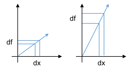
#
# * Consider $f(x)$ vs. $x$. A given $\delta x$ added to $x$ will result in some $\delta f$ added to $f$. That is, $x+\delta x\rightarrow f + \delta f$.
# * The condition number relates sensitivity of errors in $x$ to errors in $f$.
#
#
# Matrix norm (induced):
# * $\|A\| = \max(\|Ax\|/\|x\|)$ for all $x$.
# * Think of this as the maximum factor by which a matrix stretches a vector.
# ### Condition number
#
# * Consider $f(x)$ vs. $x$. A given $\delta x$ added to $x$ will result in some $\delta f$ added to $f$. That is, $x+\delta x\rightarrow f + \delta f$.
# * The condition number relates sensitivity of errors in $x$ to errors in $f$.
#  #
#
# #### Example
#
# $$\left[ \begin{array}{cc}
# 1 & 1 \\
# 1 & 1.0001 \\
# \end{array} \right] \left[\begin{array}{c} x_1 \\ x_2 \end{array}\right] =
# \left[\begin{array}{c} 2 \\ 2.0001 \end{array}\right]$$
#
# * The solution to this is $(1,1)$.
# * But if we change the 2.0001 to 2.0000, the solution is $(2,0)$.
# * A small change in $b$ gives a large change in $x$.
# * The condition number of $A$ is about 40,000.
# In[1]:
import numpy as np
A = np.array([[1,1],[1,1.0001]])
b = np.array([2,2.0000])
x = np.linalg.solve(A,b)
print('x = ', x)
print('Condition number of A = ', np.linalg.cond(A))
# #### Evaluate the condition number
#
# Note, a property of norms gives $\|Ax\| \le \|A\|\|x\|$
#
# * $Ax=b \rightarrow \|b\|\le\|A\|\|x\|$.
# * $A(x+\delta x) = b+\delta b \rightarrow A\delta x = \delta b$
# * So, $\delta x = A^{-1}\delta b$
# * $\rightarrow \|\delta x\| \le \|A^{-1}\|\|\delta b\|$.
# * Combining expressions for $\|b\|$ and $\|\delta x\|$, we get:
# $$\|b\|\|\delta x\| \le \|A\|\|x\|\|A^{-1}\|\|\delta b\| = \|A\|\|A^{-1}\|x\|\|\delta b\|$$
#
# So,
#
# $$\frac{\|\delta x\|}{\|x\|} \le \|A\|\|A^{-1}\|\frac{\|\delta b\|}{\|b\|}$$
#
# * Here, $\|A\|\|A^{-1}\|$ is the condition number $C(A)$.
# * This equation means (the relative change in $x$) $\le$ $C(A) \cdot$ (the relative change in $b$).
#
# In terms of relative error (RE): $$RE_x = C(A)\cdot RE_b.$$
# * If $C(A) = 1/\epsilon_{mach}$, and $RE_{b}=\epsilon_{mach}$, then $RE_x=1$. That is $RE_x$ = 100% error.
# * **When doing matrix inversion, you can expect to lose 1 digit of accuracy for each order of magnitude of $C(A)$.**
# * So, if $C(A) = 1000$, you will lose 3 digits of accuracy (out of 16).
#
#
# #### Example
#
# $$\left[ \begin{array}{cc}
# 1 & 1 \\
# 1 & 1.0001 \\
# \end{array} \right] \left[\begin{array}{c} x_1 \\ x_2 \end{array}\right] =
# \left[\begin{array}{c} 2 \\ 2.0001 \end{array}\right]$$
#
# * The solution to this is $(1,1)$.
# * But if we change the 2.0001 to 2.0000, the solution is $(2,0)$.
# * A small change in $b$ gives a large change in $x$.
# * The condition number of $A$ is about 40,000.
# In[1]:
import numpy as np
A = np.array([[1,1],[1,1.0001]])
b = np.array([2,2.0000])
x = np.linalg.solve(A,b)
print('x = ', x)
print('Condition number of A = ', np.linalg.cond(A))
# #### Evaluate the condition number
#
# Note, a property of norms gives $\|Ax\| \le \|A\|\|x\|$
#
# * $Ax=b \rightarrow \|b\|\le\|A\|\|x\|$.
# * $A(x+\delta x) = b+\delta b \rightarrow A\delta x = \delta b$
# * So, $\delta x = A^{-1}\delta b$
# * $\rightarrow \|\delta x\| \le \|A^{-1}\|\|\delta b\|$.
# * Combining expressions for $\|b\|$ and $\|\delta x\|$, we get:
# $$\|b\|\|\delta x\| \le \|A\|\|x\|\|A^{-1}\|\|\delta b\| = \|A\|\|A^{-1}\|x\|\|\delta b\|$$
#
# So,
#
# $$\frac{\|\delta x\|}{\|x\|} \le \|A\|\|A^{-1}\|\frac{\|\delta b\|}{\|b\|}$$
#
# * Here, $\|A\|\|A^{-1}\|$ is the condition number $C(A)$.
# * This equation means (the relative change in $x$) $\le$ $C(A) \cdot$ (the relative change in $b$).
#
# In terms of relative error (RE): $$RE_x = C(A)\cdot RE_b.$$
# * If $C(A) = 1/\epsilon_{mach}$, and $RE_{b}=\epsilon_{mach}$, then $RE_x=1$. That is $RE_x$ = 100% error.
# * **When doing matrix inversion, you can expect to lose 1 digit of accuracy for each order of magnitude of $C(A)$.**
# * So, if $C(A) = 1000$, you will lose 3 digits of accuracy (out of 16).