#!/usr/bin/env python
# coding: utf-8
# $$\newcommand{\xv}{\mathbf{x}}
# \newcommand{\Xv}{\mathbf{X}}
# \newcommand{\yv}{\mathbf{y}}
# \newcommand{\Yv}{\mathbf{Y}}
# \newcommand{\zv}{\mathbf{z}}
# \newcommand{\av}{\mathbf{a}}
# \newcommand{\Wv}{\mathbf{W}}
# \newcommand{\wv}{\mathbf{w}}
# \newcommand{\betav}{\mathbf{\beta}}
# \newcommand{\gv}{\mathbf{g}}
# \newcommand{\Hv}{\mathbf{H}}
# \newcommand{\dv}{\mathbf{d}}
# \newcommand{\Vv}{\mathbf{V}}
# \newcommand{\vv}{\mathbf{v}}
# \newcommand{\Uv}{\mathbf{U}}
# \newcommand{\uv}{\mathbf{u}}
# \newcommand{\tv}{\mathbf{t}}
# \newcommand{\Tv}{\mathbf{T}}
# \newcommand{\Sv}{\mathbf{S}}
# \newcommand{\Gv}{\mathbf{G}}
# \newcommand{\zv}{\mathbf{z}}
# \newcommand{\Zv}{\mathbf{Z}}
# \newcommand{\Norm}{\mathcal{N}}
# \newcommand{\muv}{\boldsymbol{\mu}}
# \newcommand{\sigmav}{\boldsymbol{\sigma}}
# \newcommand{\phiv}{\boldsymbol{\phi}}
# \newcommand{\Phiv}{\boldsymbol{\Phi}}
# \newcommand{\Sigmav}{\boldsymbol{\Sigma}}
# \newcommand{\Lambdav}{\boldsymbol{\Lambda}}
# \newcommand{\half}{\frac{1}{2}}
# \newcommand{\argmax}[1]{\underset{#1}{\operatorname{argmax}}}
# \newcommand{\argmin}[1]{\underset{#1}{\operatorname{argmin}}}
# \newcommand{\dimensionbar}[1]{\underset{#1}{\operatorname{|}}}
# \newcommand{\grad}{\mathbf{\nabla}}
# \newcommand{\ebx}[1]{e^{\betav_{#1}^T \xv_n}}
# \newcommand{\eby}[1]{e^{y_{n,#1}}}
# \newcommand{\Tiv}{\mathbf{Ti}}
# \newcommand{\Fv}{\mathbf{F}}
# \newcommand{\ones}[1]{\mathbf{1}_{#1}}
# $$
# # Introduction to Reinforcement Learning
# ## Concepts
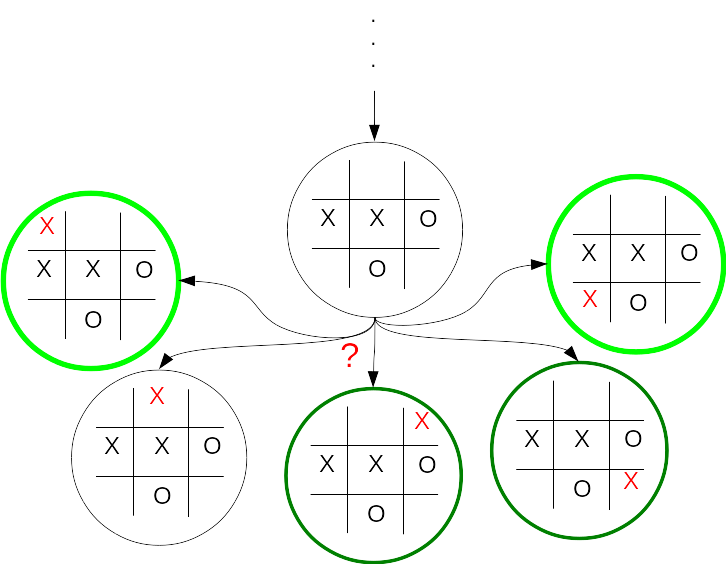
# Imagine a position in a tic-tac-toe game (knots and crosses).
# How do you choose the best next action?
#
# 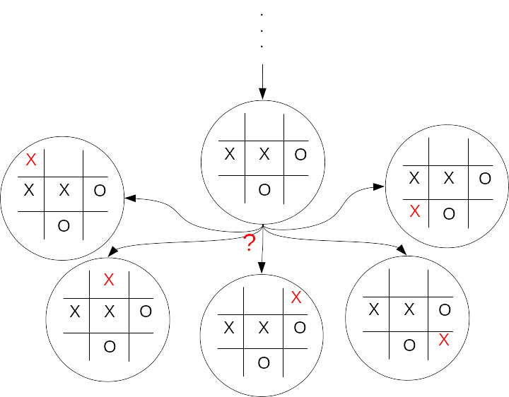 #
# Which are you most likely to win from?
# Guess at how likely you are to win from each state. Is a win
# definite, likely, or maybe?
#
#
#
# Which are you most likely to win from?
# Guess at how likely you are to win from each state. Is a win
# definite, likely, or maybe?
#
#  # ## States and Actions
# Set of possible states, $\mathcal{S}$.
#
# * Can be discrete values ($|\mathcal{S}| < \infty$)
# * Tic-Tac-Toe game positions
# * Position in a maze
# * Sequence of steps in a plan
# * Can be continuous values ($|\mathcal{S}| = \infty$)
# * Joint angles of a robot arm
# * Position and velocity of a race car
# * Parameter values for a network routing strategy
#
# Set of possible actions, $\mathcal{A}$.
#
# * Can be discrete values ($|\mathcal{A}| < \infty$)
# * Next moves in Tic-Tac-Toe
# * Directions to step in a maze
# * Rearrangements of a sequence of steps in a plan
# * Can be continuous values ($|\mathcal{A}| = \infty$)
# * Torques to apply to the joints of a robot arm
# * Fuel rate and turning torque in a race car
# * Settings of parameter values for a network routing strategy
# ## Values
# We want to choose the action that we predict will result in the best
# possible future from the current state. Need a value that
# represents the future outcome.
#
# What should the value represent?
#
# * Tic-Tac-Toe: Likelihood of winning from a game position.
# * Maze: Number of steps to reach the goal.
# * Plan: Efficiency in time and cost of accomplishing the objective for particular rearrangment of steps in a plan.
# * Robot: Energy required to move the gripper on a robot arm to a destination.
# * Race car: Time to reach the finish line.
# * Network routing: Throughput.
#
# With the correct values, multi-step decision problems are reduced
# to single-step decision problems. Just pick action with best
# value. Guaranteed to find optimal multi-step solution (dynamic programming).
#
# The utility or cost of a single action taken from a state is the **reinforcement**
# for that action from that state. The value of that state-action is
# the expected value of the full **return** or the sum of reinforcements that will follow
# when that action is taken.
#
#
# ## States and Actions
# Set of possible states, $\mathcal{S}$.
#
# * Can be discrete values ($|\mathcal{S}| < \infty$)
# * Tic-Tac-Toe game positions
# * Position in a maze
# * Sequence of steps in a plan
# * Can be continuous values ($|\mathcal{S}| = \infty$)
# * Joint angles of a robot arm
# * Position and velocity of a race car
# * Parameter values for a network routing strategy
#
# Set of possible actions, $\mathcal{A}$.
#
# * Can be discrete values ($|\mathcal{A}| < \infty$)
# * Next moves in Tic-Tac-Toe
# * Directions to step in a maze
# * Rearrangements of a sequence of steps in a plan
# * Can be continuous values ($|\mathcal{A}| = \infty$)
# * Torques to apply to the joints of a robot arm
# * Fuel rate and turning torque in a race car
# * Settings of parameter values for a network routing strategy
# ## Values
# We want to choose the action that we predict will result in the best
# possible future from the current state. Need a value that
# represents the future outcome.
#
# What should the value represent?
#
# * Tic-Tac-Toe: Likelihood of winning from a game position.
# * Maze: Number of steps to reach the goal.
# * Plan: Efficiency in time and cost of accomplishing the objective for particular rearrangment of steps in a plan.
# * Robot: Energy required to move the gripper on a robot arm to a destination.
# * Race car: Time to reach the finish line.
# * Network routing: Throughput.
#
# With the correct values, multi-step decision problems are reduced
# to single-step decision problems. Just pick action with best
# value. Guaranteed to find optimal multi-step solution (dynamic programming).
#
# The utility or cost of a single action taken from a state is the **reinforcement**
# for that action from that state. The value of that state-action is
# the expected value of the full **return** or the sum of reinforcements that will follow
# when that action is taken.
#
# 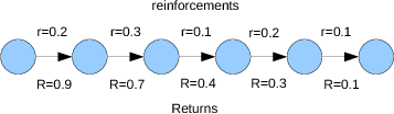 #
# Say we are in state $s_t$ at time $t$. Upon taking action $a_t$
# from that state we observe the one step reinforcement $r_{t+1}$,
# and the next state $s_{t+1}$.
#
# Say this continues until we reach a goal state, $K$ steps later.
# What is the return $R_t$ from state $s_t$?
#
# $$
# \begin{align*}
# R_t = \sum_{k=0}^K r_{t+k+1}
# \end{align*}
# $$
#
#
# Use the returns to choose the best action.
#
#
#
# Say we are in state $s_t$ at time $t$. Upon taking action $a_t$
# from that state we observe the one step reinforcement $r_{t+1}$,
# and the next state $s_{t+1}$.
#
# Say this continues until we reach a goal state, $K$ steps later.
# What is the return $R_t$ from state $s_t$?
#
# $$
# \begin{align*}
# R_t = \sum_{k=0}^K r_{t+k+1}
# \end{align*}
# $$
#
#
# Use the returns to choose the best action.
#
# 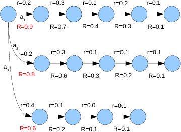 #
# Right...are we maximizing or minimizing? What does the
# reinforcement represent? Let's say it is energy used that we want
# to minimize. $a_1$, $a_2$, or $a_3$?
#
# Where do the values come from?
#
# * Write the code to calculate them.
# * Usually not possible. If you can do this for your problem, why are you considering machine learning? Might be able to do this for Tic-Tac-Toe.
# * Use dynamic programming.
# * Usually not possible. Requires knowledge of the probabilities of transitions between all states for all actions.
# * Learn from examples, lots of examples. Lots of 5-tuples: state, action, reinforcement, next state, next action ($s_t, a_t, r_{t+1}, s_{t+1}, a_{t+1}$).
# * **Monte Carlo:** Assign to each state-action pair an average of the observed returns: $ \;\;\;\text{value}(s_t,a_t) \approx \text{mean of } R(s_t,a_t)$
# * **Temporal Difference (TD):** Using $\text{value}(s_{t+1},a_{t+1})$ as estimate of return from next state, update current state-action value: $\;\;\; \text{value}(s_t,a_t) \approx r_{t+1} + \text{value}(s_{t+1},a_{t+1})$
#
# What is the estimate of the return $R$ from state B?
#
#
#
# Right...are we maximizing or minimizing? What does the
# reinforcement represent? Let's say it is energy used that we want
# to minimize. $a_1$, $a_2$, or $a_3$?
#
# Where do the values come from?
#
# * Write the code to calculate them.
# * Usually not possible. If you can do this for your problem, why are you considering machine learning? Might be able to do this for Tic-Tac-Toe.
# * Use dynamic programming.
# * Usually not possible. Requires knowledge of the probabilities of transitions between all states for all actions.
# * Learn from examples, lots of examples. Lots of 5-tuples: state, action, reinforcement, next state, next action ($s_t, a_t, r_{t+1}, s_{t+1}, a_{t+1}$).
# * **Monte Carlo:** Assign to each state-action pair an average of the observed returns: $ \;\;\;\text{value}(s_t,a_t) \approx \text{mean of } R(s_t,a_t)$
# * **Temporal Difference (TD):** Using $\text{value}(s_{t+1},a_{t+1})$ as estimate of return from next state, update current state-action value: $\;\;\; \text{value}(s_t,a_t) \approx r_{t+1} + \text{value}(s_{t+1},a_{t+1})$
#
# What is the estimate of the return $R$ from state B?
#
# 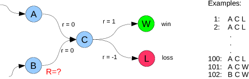 #
# * **Monte Carlo:** $\text{mean of } R(s_t,a_t)$ = 1, a prediction of a win
# * **Temporal Difference (TD):** $r_{t+1} + \text{value}(s_{t+1},a_{t+1}) = 0 + (100(-1) + 2(1))/100 = -0.98$, a very likely loss
# * What do you do? The green pill or the red pill?
# * TD takes advantage of the cached experience given in the value learned for State C.
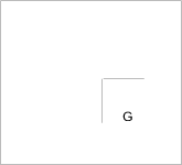
# ## Example: Maze
#
# Here is a simple maze.
#
#
#
# * **Monte Carlo:** $\text{mean of } R(s_t,a_t)$ = 1, a prediction of a win
# * **Temporal Difference (TD):** $r_{t+1} + \text{value}(s_{t+1},a_{t+1}) = 0 + (100(-1) + 2(1))/100 = -0.98$, a very likely loss
# * What do you do? The green pill or the red pill?
# * TD takes advantage of the cached experience given in the value learned for State C.
# ## Example: Maze
#
# Here is a simple maze.
#
#  #
# From any position, how do you decide whether to move up, right, down, or left?
#
# Right. Need an estimate of the number of steps to reach the
# goal. This will be the return $R$. How do we formulate this in terms of
# reinforcements?
#
# Yep. $r_t = 1$ for every step. Then $R_t = \sum_{k=0}^K r_{t+k+1}$ will sum of those 1's to produce the number of steps to
# goal from each state.
#
# The Monte-carlo way will assign value as average of number of steps to goal from each
# starting state tried.
#
# The TD way will update value based on (1 + estimated value from next state).
#
#
# Should we do Monte-Carlo update or Temporal-Difference updates? Take a look at this comparison on the maze problem.
# # State-Action Value Function as a Table
# ## Tabular Function
# Recall that the state-action value function is a function of
# both state and action and its value is a prediction of the
# expected sum of future reinforcements.
#
# We will call the state-action value function $Q$, after
# [Learning from Delayed Rewards](http://www.cs.rhul.ac.uk/~chrisw/thesis.html), by C. Watkins, PhD
# Thesis, University of Cambridge, Cambridge, UK, 1989.
#
# We can select our current belief of what the optimal action, $a_t^o$, is in state $s_t$ by
#
# $$
# \begin{align*}
# a_t^o = \argmax{a} Q(s_t,a)
# \end{align*}
# $$
#
# or
#
# $$
# \begin{align*}
# a_t^o = \argmin{a} Q(s_t,a)
# \end{align*}
# $$
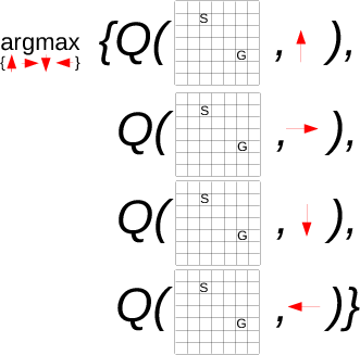
# ## Tabular Q for the Maze Problem
# ### Representing the Q Table
# For the maze world,
#
#
# $$
# \begin{align*}
# a_t^o = \argmin{a} Q(s_t,a)
# \end{align*}
# $$
#
#
# looks like (argmax should be argmin)
#
#
#
# From any position, how do you decide whether to move up, right, down, or left?
#
# Right. Need an estimate of the number of steps to reach the
# goal. This will be the return $R$. How do we formulate this in terms of
# reinforcements?
#
# Yep. $r_t = 1$ for every step. Then $R_t = \sum_{k=0}^K r_{t+k+1}$ will sum of those 1's to produce the number of steps to
# goal from each state.
#
# The Monte-carlo way will assign value as average of number of steps to goal from each
# starting state tried.
#
# The TD way will update value based on (1 + estimated value from next state).
#
#
# Should we do Monte-Carlo update or Temporal-Difference updates? Take a look at this comparison on the maze problem.
# # State-Action Value Function as a Table
# ## Tabular Function
# Recall that the state-action value function is a function of
# both state and action and its value is a prediction of the
# expected sum of future reinforcements.
#
# We will call the state-action value function $Q$, after
# [Learning from Delayed Rewards](http://www.cs.rhul.ac.uk/~chrisw/thesis.html), by C. Watkins, PhD
# Thesis, University of Cambridge, Cambridge, UK, 1989.
#
# We can select our current belief of what the optimal action, $a_t^o$, is in state $s_t$ by
#
# $$
# \begin{align*}
# a_t^o = \argmax{a} Q(s_t,a)
# \end{align*}
# $$
#
# or
#
# $$
# \begin{align*}
# a_t^o = \argmin{a} Q(s_t,a)
# \end{align*}
# $$
# ## Tabular Q for the Maze Problem
# ### Representing the Q Table
# For the maze world,
#
#
# $$
# \begin{align*}
# a_t^o = \argmin{a} Q(s_t,a)
# \end{align*}
# $$
#
#
# looks like (argmax should be argmin)
#
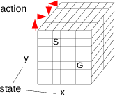
#  #
# A bit more mathematically, let the current state be given by
# position in $x$ and $y$ coordinates and actions are integers 1 to
# 4. Then
#
# $$
# \begin{align*}
# a_t^o = \argmin{a\in \{1,2,3,4\}} Q\left ((x,y), a\right )
# \end{align*}
# $$
#
#
# Now, let's try to do this in python.
#
# How do we implement the Q function? For the maze problem, we know we can
#
# * enumerate all the states (positions) the set of which is finite ($10\cdot 10$),
# * enumerate all actions, the set of which is finite (4),
# * calculate the new state from the old state and an action, and
# * represent in memory all state-action combinations ($10\cdot 10\cdot 4$).
#
# So, let's just store the Q function in table form.
#
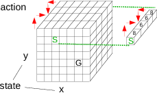
# The Q table will need three dimensions, for $x$, $y$, and the action.
#
#
#
# A bit more mathematically, let the current state be given by
# position in $x$ and $y$ coordinates and actions are integers 1 to
# 4. Then
#
# $$
# \begin{align*}
# a_t^o = \argmin{a\in \{1,2,3,4\}} Q\left ((x,y), a\right )
# \end{align*}
# $$
#
#
# Now, let's try to do this in python.
#
# How do we implement the Q function? For the maze problem, we know we can
#
# * enumerate all the states (positions) the set of which is finite ($10\cdot 10$),
# * enumerate all actions, the set of which is finite (4),
# * calculate the new state from the old state and an action, and
# * represent in memory all state-action combinations ($10\cdot 10\cdot 4$).
#
# So, let's just store the Q function in table form.
#
# The Q table will need three dimensions, for $x$, $y$, and the action.
#
#  #
# How do we look up the Q values for a state?
#
#
#
# How do we look up the Q values for a state?
#
#  #
# Q values are steps to goal, so we are minimizing. Select right or down action.
#
# We are finally ready for python. How can we make a three-dimensional table of Q values, if $x$ and $y$ have 10 possible values
# and we have 4 actions?
#
# import numpy as np
# Q = np.zeros((10, 10, 4))
#
# How should we initialize the table? Above line initializes all values to be zero. What effect will
# this have as Q values for actions taken are updated to estimate steps to goal?
#
# Actions not yet tried will have lowest (0) Q value. Forces
# the agent to try all actions from all states---lots of **exploration**.
# ### Updating the Q Table Using Temporal-Difference Updates
# What must we do after observing $s_t$, $a_t$, $r_{t+1}$, $s_{t+1}$, and $a_{t+1}$?
#
# Calculate the temporal-difference error $r_{t+1} + Q(s_{t+1},a_{t+1}) - Q(s_t,a_t)$ and use it to
# update the Q value stored for $s_t$ and $a_t$:
#
# $$
# \begin{align*}
# Q(s_t,a_t) = Q(s_t,a_t) + \rho (r_{t+1} + Q(s_{t+1},a_{t+1}) - Q(s_t,a_t))
# \end{align*}
# $$
#
#
# And, in python? Assume position, or state, $(2, 3)$ is implemented as ''state = np.array([2, 3])''.
#
# r = 1
# Qold = Q[stateOld[0], stateOld[1], actionOld]
# Qnew = Q[state[0], state[1], action]
# TDError = r + Qnew - Qold
# Q[stateOld[0], stateOld[1], actionOld] = Qold + rho * TDError
#
#
# This is performed for every pair of steps $t$ and $t+1$, until the final step,
# which must be handled differently. There is no $s_{t+1}$.
# The update
#
# $$
# \begin{align*}
# Q(s_t,a_t) = Q(s_t,a_t) + \rho (r_{t+1} + Q(s_{t+1},a_{t+1}) - Q(s_t,a_t))
# \end{align*}
# $$
#
# becomes
#
# $$
# \begin{align*}
# Q(s_t,a_t) = Q(s_t,a_t) + \rho (r_{t+1} - Q(s_t,a_t))
# \end{align*}
# $$
#
#
# In python, add a test for being at the goal. Let ''maze'' be character array containing a ''G'' at the
# goal position.
#
# r = 1
# Qold = Q[stateOld[0], stateOld[1], actionOld]
# Qnew = Q[state[0], state[1], action]
#
# if (maze[state[0]+1,state[1]+1] == 'G'):
# TDerror = r - Qold
# else:
# TDerror = r + Qnew - Qold
#
# Q[stateOld[0], stateOld[1], actionOld] = Qold + rho * TDerror
#
#
# To choose the best action for state $(x, y)$ stored in variable state,
# just need to do
#
# a = np.argmin(Q[state[0], state[1], :])
#
# and if we store the available actions as
#
# actions = np.array([[0, 1], [1, 0], [0, -1], [-1, 0]])
#
# then the update to state based on action a is done by
#
# state = state + actions[a, :]
# ## The Agent-Environment Interaction Loop
# For our agent to interact with its world, we must implement the steps
#
# 1. Initialize Q.
# 1. Choose random, non-goal, state.
# 1. Repeat:
# 1. If at goal,
# 1. Update Qold with TD error (1 - Qold)
# 1. Pick new random state
# 1. Otherwise (not at goal),
# 1. Select next action.
# 1. If not first step, update Qold with TD error (1 + Qnew - Qold)
# 1. Shift current state and action to old ones.
# 1. Apply action to get new state.
#
# In Python it would look something like the following for a 10x10 maze.
#
# Q = np.zeros((10,10,4)) # 1.
# s = np.random.randint(0,10,2) # 2.
# for step in xrange(10000): # 3. (or forever)
# if isGoal(s): # 3.A.
# Q[sOld[0],sOld[1],aOld] += # 3.A.a
# rho * (1 - Q[sOld[0],sOld[1],aOld])
# s = np.random.randint(0,10,2) # 3.A.b
# else: # 3.B
# a = np.argmin(Q[s[0],s[1],:]) # 3.B.a
# if steps > 1:
# Q[sOld[0],sOld[1],aOld] += # 3.B.b
# rho * (1 + Q[s[0],s[1],a] - Q[sOld[0],sOld[1],aOld])
# sOld, aOld = s, a # 3.B.c
# s += actions[a,:] # 3.B.d
# # Python Solution of the Maze Problem
# First, we start with a text file that specifies a maze. Let's use the cell magic %%writefile to make the maze file.
# In[14]:
import numpy as np
import matplotlib.pyplot as plt
from mpl_toolkits.mplot3d import Axes3D
# In[15]:
get_ipython().run_cell_magic('writefile', 'maze1.txt', '************\n* *\n* *\n* *\n* *\n* *\n* ***** *\n* * *\n* G * *\n* * *\n* *\n************\n')
# In[16]:
get_ipython().run_cell_magic('writefile', 'maze1.txt', '************\n* *\n* *\n* * *\n* * *\n* * *\n* **** *\n* * G* *\n* * * *\n* * * *\n* *\n************\n')
# In[17]:
with open('maze1.txt') as f:
for line in f:
print(line.strip())
# In[18]:
mazelist = []
with open('maze1.txt') as f:
for line in f:
mazelist.append(line.strip())
mazelist
# In[19]:
maze = np.array(mazelist).view('U1').reshape((len(mazelist), len(mazelist[0])))
print(maze.shape)
maze
# In[20]:
for i in range(maze.shape[0]):
for j in range(maze.shape[1]):
print(maze[i,j],end='')
print()
# Need some functions, one to draw the Q surface, over the two-dimensional state space (position in the maze), and one to select an action given the Q surface.
# In[21]:
### Draw Q surface, showing minimum Q value for each state
def showQ(Q, title, ax):
(m, n, _) = Q.shape
gridsize = max(m, n)
rows = np.floor(np.linspace(0, m - 0.5, gridsize))
cols = np.floor(np.linspace(0, n - 0.5, gridsize))
ygrid, xgrid = np.meshgrid(rows, cols, indexing='ij')
points = np.vstack((ygrid.flat, xgrid.flat))
Qmins = [np.min( Q[int(s1), int(s2), :]) for (s1, s2) in zip(points[0, :], points[1, :])]
Qmins = np.asarray(Qmins).reshape(xgrid.shape)
ax.plot_surface(xgrid, ygrid, Qmins, color='yellow')
plt.ylim(m - 1 + 0.5, 0 - 0.5)
ax.set_zlabel('Qmin')
ax.set_title(f'Min {np.min(Qmins):.1f} Max {np.max(Qmins):.1f}')
### Show current policy
def showPolicy(Q):
(m, n, _) = Q.shape
bestactions = np.argmin(Q, axis=2)
prow, pcol = np.meshgrid(np.arange(m), np.arange(n), indexing='ij')
arrowrow = actions[:, 0][bestactions]
arrowcol = actions[:, 1][bestactions]
plt.quiver(pcol, prow, arrowcol, -arrowrow)
walls_row, walls_col = np.where(maze[1:-1, 1:-1] == '*')
plt.plot(walls_col, walls_row, 'ro', ms=15, alpha=0.5)
goal_row, goal_col = np.where(maze[1:-1, 1:-1] == 'G')
plt.plot(goal_col, goal_row, 'go', ms=15, alpha=0.5)
plt.ylim(m - 1 + 0.5, 0 - 0.5)
plt.xlim(0 - 0.5, n - 1 + 0.5)
# Construct arrays to hold the tabular Q values updated by temporal differences, and one to hold Q values updated by Monte Carlo. Set Q values to *np.inf* for invalid actions. We have four possible actions from each position.
# In[22]:
m, n = maze.shape
m -= 2 # for ceiling and floor
n -= 2 # for walls
Q = np.zeros((m, n, 4))
Qmc = np.zeros((m, n, 4))
actions = np.array([[0, 1], [1, 0], [0, -1], [-1, 0]]) # changes in row and column position of RL agent
### Set Q value of invalid actions to np.inf
for mi in range(m):
for ni in range(n):
for ai in range(4):
r = mi + actions[ai, 0]
c = ni + actions[ai, 1]
if maze[r + 1, c + 1] == '*': # showing ai was invalid action
Q[mi, ni, ai] = np.inf
Qmc[mi, ni, ai] = np.inf
# Now for some parameters. Let's run for 50,000 interactions with maze environment, so 50,000 updates, and let $\rho$, the learning rate, be 0.1 and $\epsilon$, the random action probability, be 0.01.
# In[23]:
nSteps = 100000
rho = 0.1
epsilon = 0.2
# Now we need to keep a history, or trace, of positions and reinforcement, to be used to update the MC version of Q.
# In[24]:
trace = np.zeros((nSteps, 3)) # for x, y, and a
# In[25]:
from IPython.display import display, clear_output
# Need some initializations before starting the loop.
# In[26]:
fig = plt.figure(figsize=(10, 10))
s = np.array([1, 1]) # start position
a = 1 #first action (index)
trials = []
steps = 0
goals = 0
for step in range(nSteps):
trace[steps, :] = s.tolist() + [a]
here = maze[s[0] + 1, s[1] + 1]
if here == 'G':
# Found the Goal!
goals += 1
Q[s[0], s[1], a] = 0
if steps > 0:
Q[sold[0], sold[1], aold] += rho * (1 - Q[sold[0], sold[1], aold])
# Monte Carlo update
cost = 0
for sai in range(steps, -1, -1):
r, c, act = trace[sai, :]
r, c, act = int(r), int(c), int(act)
Qmc[r, c, act] = (1 - rho) * Qmc[r, c, act] + rho * cost
cost += 1
s = np.array([np.random.randint(0, m), np.random.randint(0, n)])
#sold = []
trials.append(steps)
else:
# Not goal
steps += 1
Qfunc = Q # Qfunc = Qmc # to use Monte Carlo policy to drive behavior
# Pick next action a
if np.random.uniform() < epsilon:
validActions = [a for (i, a) in enumerate(range(4)) if not np.isinf(Qfunc[s[0], s[1], i])]
a = np.random.choice(validActions)
else:
a = np.argmin(Qfunc[s[0], s[1], :])
if steps > 1:
Q[sold[0], sold[1], aold] += rho * (1 + Q[s[0], s[1], a] - Q[sold[0], sold[1], aold])
sold = s
aold = a
s = s + actions[a, :]
if (here == 'G' and goals % 100 == 0):
fig.clf()
ax = fig.add_subplot(3, 2, 1, projection='3d')
showQ(Q, 'TD', ax)
ax = fig.add_subplot(3, 2, 2, projection='3d')
showQ(Qmc, 'Monte Carlo', ax)
plt.subplot(3, 2, 3)
showPolicy(Q)
plt.title('Q Policy')
plt.subplot(3, 2, 4)
showPolicy(Qmc)
plt.title('Monte Carlo Q Policy')
plt.subplot(3, 2, 5)
plt.plot(trace[:steps + 1, 1], trace[:steps + 1, 0], 'o-')
plt.plot(trace[0, 1], trace[0, 0], 'ro')
plt.xlim(0 - 0.5, 9 + 0.5)
plt.ylim(9 + 0.5, 0 - 0.5)
plt.title('Most Recent Trial')
plt.subplot(3, 2, 6)
plt.plot(trials, '-')
plt.xlabel('Trial')
plt.ylabel('Steps to Goal')
clear_output(wait=True)
display(fig);
if here == 'G':
steps = 0
clear_output(wait=True)
# In[ ]:
# In[ ]:
#
# Q values are steps to goal, so we are minimizing. Select right or down action.
#
# We are finally ready for python. How can we make a three-dimensional table of Q values, if $x$ and $y$ have 10 possible values
# and we have 4 actions?
#
# import numpy as np
# Q = np.zeros((10, 10, 4))
#
# How should we initialize the table? Above line initializes all values to be zero. What effect will
# this have as Q values for actions taken are updated to estimate steps to goal?
#
# Actions not yet tried will have lowest (0) Q value. Forces
# the agent to try all actions from all states---lots of **exploration**.
# ### Updating the Q Table Using Temporal-Difference Updates
# What must we do after observing $s_t$, $a_t$, $r_{t+1}$, $s_{t+1}$, and $a_{t+1}$?
#
# Calculate the temporal-difference error $r_{t+1} + Q(s_{t+1},a_{t+1}) - Q(s_t,a_t)$ and use it to
# update the Q value stored for $s_t$ and $a_t$:
#
# $$
# \begin{align*}
# Q(s_t,a_t) = Q(s_t,a_t) + \rho (r_{t+1} + Q(s_{t+1},a_{t+1}) - Q(s_t,a_t))
# \end{align*}
# $$
#
#
# And, in python? Assume position, or state, $(2, 3)$ is implemented as ''state = np.array([2, 3])''.
#
# r = 1
# Qold = Q[stateOld[0], stateOld[1], actionOld]
# Qnew = Q[state[0], state[1], action]
# TDError = r + Qnew - Qold
# Q[stateOld[0], stateOld[1], actionOld] = Qold + rho * TDError
#
#
# This is performed for every pair of steps $t$ and $t+1$, until the final step,
# which must be handled differently. There is no $s_{t+1}$.
# The update
#
# $$
# \begin{align*}
# Q(s_t,a_t) = Q(s_t,a_t) + \rho (r_{t+1} + Q(s_{t+1},a_{t+1}) - Q(s_t,a_t))
# \end{align*}
# $$
#
# becomes
#
# $$
# \begin{align*}
# Q(s_t,a_t) = Q(s_t,a_t) + \rho (r_{t+1} - Q(s_t,a_t))
# \end{align*}
# $$
#
#
# In python, add a test for being at the goal. Let ''maze'' be character array containing a ''G'' at the
# goal position.
#
# r = 1
# Qold = Q[stateOld[0], stateOld[1], actionOld]
# Qnew = Q[state[0], state[1], action]
#
# if (maze[state[0]+1,state[1]+1] == 'G'):
# TDerror = r - Qold
# else:
# TDerror = r + Qnew - Qold
#
# Q[stateOld[0], stateOld[1], actionOld] = Qold + rho * TDerror
#
#
# To choose the best action for state $(x, y)$ stored in variable state,
# just need to do
#
# a = np.argmin(Q[state[0], state[1], :])
#
# and if we store the available actions as
#
# actions = np.array([[0, 1], [1, 0], [0, -1], [-1, 0]])
#
# then the update to state based on action a is done by
#
# state = state + actions[a, :]
# ## The Agent-Environment Interaction Loop
# For our agent to interact with its world, we must implement the steps
#
# 1. Initialize Q.
# 1. Choose random, non-goal, state.
# 1. Repeat:
# 1. If at goal,
# 1. Update Qold with TD error (1 - Qold)
# 1. Pick new random state
# 1. Otherwise (not at goal),
# 1. Select next action.
# 1. If not first step, update Qold with TD error (1 + Qnew - Qold)
# 1. Shift current state and action to old ones.
# 1. Apply action to get new state.
#
# In Python it would look something like the following for a 10x10 maze.
#
# Q = np.zeros((10,10,4)) # 1.
# s = np.random.randint(0,10,2) # 2.
# for step in xrange(10000): # 3. (or forever)
# if isGoal(s): # 3.A.
# Q[sOld[0],sOld[1],aOld] += # 3.A.a
# rho * (1 - Q[sOld[0],sOld[1],aOld])
# s = np.random.randint(0,10,2) # 3.A.b
# else: # 3.B
# a = np.argmin(Q[s[0],s[1],:]) # 3.B.a
# if steps > 1:
# Q[sOld[0],sOld[1],aOld] += # 3.B.b
# rho * (1 + Q[s[0],s[1],a] - Q[sOld[0],sOld[1],aOld])
# sOld, aOld = s, a # 3.B.c
# s += actions[a,:] # 3.B.d
# # Python Solution of the Maze Problem
# First, we start with a text file that specifies a maze. Let's use the cell magic %%writefile to make the maze file.
# In[14]:
import numpy as np
import matplotlib.pyplot as plt
from mpl_toolkits.mplot3d import Axes3D
# In[15]:
get_ipython().run_cell_magic('writefile', 'maze1.txt', '************\n* *\n* *\n* *\n* *\n* *\n* ***** *\n* * *\n* G * *\n* * *\n* *\n************\n')
# In[16]:
get_ipython().run_cell_magic('writefile', 'maze1.txt', '************\n* *\n* *\n* * *\n* * *\n* * *\n* **** *\n* * G* *\n* * * *\n* * * *\n* *\n************\n')
# In[17]:
with open('maze1.txt') as f:
for line in f:
print(line.strip())
# In[18]:
mazelist = []
with open('maze1.txt') as f:
for line in f:
mazelist.append(line.strip())
mazelist
# In[19]:
maze = np.array(mazelist).view('U1').reshape((len(mazelist), len(mazelist[0])))
print(maze.shape)
maze
# In[20]:
for i in range(maze.shape[0]):
for j in range(maze.shape[1]):
print(maze[i,j],end='')
print()
# Need some functions, one to draw the Q surface, over the two-dimensional state space (position in the maze), and one to select an action given the Q surface.
# In[21]:
### Draw Q surface, showing minimum Q value for each state
def showQ(Q, title, ax):
(m, n, _) = Q.shape
gridsize = max(m, n)
rows = np.floor(np.linspace(0, m - 0.5, gridsize))
cols = np.floor(np.linspace(0, n - 0.5, gridsize))
ygrid, xgrid = np.meshgrid(rows, cols, indexing='ij')
points = np.vstack((ygrid.flat, xgrid.flat))
Qmins = [np.min( Q[int(s1), int(s2), :]) for (s1, s2) in zip(points[0, :], points[1, :])]
Qmins = np.asarray(Qmins).reshape(xgrid.shape)
ax.plot_surface(xgrid, ygrid, Qmins, color='yellow')
plt.ylim(m - 1 + 0.5, 0 - 0.5)
ax.set_zlabel('Qmin')
ax.set_title(f'Min {np.min(Qmins):.1f} Max {np.max(Qmins):.1f}')
### Show current policy
def showPolicy(Q):
(m, n, _) = Q.shape
bestactions = np.argmin(Q, axis=2)
prow, pcol = np.meshgrid(np.arange(m), np.arange(n), indexing='ij')
arrowrow = actions[:, 0][bestactions]
arrowcol = actions[:, 1][bestactions]
plt.quiver(pcol, prow, arrowcol, -arrowrow)
walls_row, walls_col = np.where(maze[1:-1, 1:-1] == '*')
plt.plot(walls_col, walls_row, 'ro', ms=15, alpha=0.5)
goal_row, goal_col = np.where(maze[1:-1, 1:-1] == 'G')
plt.plot(goal_col, goal_row, 'go', ms=15, alpha=0.5)
plt.ylim(m - 1 + 0.5, 0 - 0.5)
plt.xlim(0 - 0.5, n - 1 + 0.5)
# Construct arrays to hold the tabular Q values updated by temporal differences, and one to hold Q values updated by Monte Carlo. Set Q values to *np.inf* for invalid actions. We have four possible actions from each position.
# In[22]:
m, n = maze.shape
m -= 2 # for ceiling and floor
n -= 2 # for walls
Q = np.zeros((m, n, 4))
Qmc = np.zeros((m, n, 4))
actions = np.array([[0, 1], [1, 0], [0, -1], [-1, 0]]) # changes in row and column position of RL agent
### Set Q value of invalid actions to np.inf
for mi in range(m):
for ni in range(n):
for ai in range(4):
r = mi + actions[ai, 0]
c = ni + actions[ai, 1]
if maze[r + 1, c + 1] == '*': # showing ai was invalid action
Q[mi, ni, ai] = np.inf
Qmc[mi, ni, ai] = np.inf
# Now for some parameters. Let's run for 50,000 interactions with maze environment, so 50,000 updates, and let $\rho$, the learning rate, be 0.1 and $\epsilon$, the random action probability, be 0.01.
# In[23]:
nSteps = 100000
rho = 0.1
epsilon = 0.2
# Now we need to keep a history, or trace, of positions and reinforcement, to be used to update the MC version of Q.
# In[24]:
trace = np.zeros((nSteps, 3)) # for x, y, and a
# In[25]:
from IPython.display import display, clear_output
# Need some initializations before starting the loop.
# In[26]:
fig = plt.figure(figsize=(10, 10))
s = np.array([1, 1]) # start position
a = 1 #first action (index)
trials = []
steps = 0
goals = 0
for step in range(nSteps):
trace[steps, :] = s.tolist() + [a]
here = maze[s[0] + 1, s[1] + 1]
if here == 'G':
# Found the Goal!
goals += 1
Q[s[0], s[1], a] = 0
if steps > 0:
Q[sold[0], sold[1], aold] += rho * (1 - Q[sold[0], sold[1], aold])
# Monte Carlo update
cost = 0
for sai in range(steps, -1, -1):
r, c, act = trace[sai, :]
r, c, act = int(r), int(c), int(act)
Qmc[r, c, act] = (1 - rho) * Qmc[r, c, act] + rho * cost
cost += 1
s = np.array([np.random.randint(0, m), np.random.randint(0, n)])
#sold = []
trials.append(steps)
else:
# Not goal
steps += 1
Qfunc = Q # Qfunc = Qmc # to use Monte Carlo policy to drive behavior
# Pick next action a
if np.random.uniform() < epsilon:
validActions = [a for (i, a) in enumerate(range(4)) if not np.isinf(Qfunc[s[0], s[1], i])]
a = np.random.choice(validActions)
else:
a = np.argmin(Qfunc[s[0], s[1], :])
if steps > 1:
Q[sold[0], sold[1], aold] += rho * (1 + Q[s[0], s[1], a] - Q[sold[0], sold[1], aold])
sold = s
aold = a
s = s + actions[a, :]
if (here == 'G' and goals % 100 == 0):
fig.clf()
ax = fig.add_subplot(3, 2, 1, projection='3d')
showQ(Q, 'TD', ax)
ax = fig.add_subplot(3, 2, 2, projection='3d')
showQ(Qmc, 'Monte Carlo', ax)
plt.subplot(3, 2, 3)
showPolicy(Q)
plt.title('Q Policy')
plt.subplot(3, 2, 4)
showPolicy(Qmc)
plt.title('Monte Carlo Q Policy')
plt.subplot(3, 2, 5)
plt.plot(trace[:steps + 1, 1], trace[:steps + 1, 0], 'o-')
plt.plot(trace[0, 1], trace[0, 0], 'ro')
plt.xlim(0 - 0.5, 9 + 0.5)
plt.ylim(9 + 0.5, 0 - 0.5)
plt.title('Most Recent Trial')
plt.subplot(3, 2, 6)
plt.plot(trials, '-')
plt.xlabel('Trial')
plt.ylabel('Steps to Goal')
clear_output(wait=True)
display(fig);
if here == 'G':
steps = 0
clear_output(wait=True)
# In[ ]:
# In[ ]: