Velocity and Acceleration of a point of a rigid body

Renato Naville Watanabe, Marcos Duarte
Laboratory of Biomechanics and Motor Control
Federal University of ABC, Brazil

Contents

• 1  Python setup
• 2  Frame of reference attached to a body
• 3  Position of a point on a rigid body
• 4  Translation of a rigid body
• 5  Angular velocity of a body
• 6  Velocity of a point with no translation
• 7  Relative velocity of a point on a rigid body to another point
• 8  Velocity of a point on rigid body translating
• 9  Acceleration of a point on a rigid body
• 10  Further reading
• 11  Video lectures on the Internet
• 12  Problems
• 13  References

This notebook shows the expressions of the velocity and acceleration of a point on rigid body, given the angular velocity of the body.

Python setup

import numpy as np
import matplotlib.pyplot as plt
%matplotlib widget
from matplotlib.animation import FuncAnimation
from matplotlib.patches import FancyArrowPatch

Frame of reference attached to a body

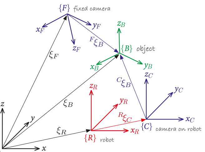
The concept of reference frame in Biomechanics and motor control is very important and central to the understanding of human motion. For example, do we see, plan and control the movement of our hand with respect to reference frames within our body or in the environment we move? Or a combination of both?
The figure below, although derived for a robotic system, illustrates well the concept that we might have to deal with multiple coordinate systems.

Figure. Multiple coordinate systems for use in robots (figure from Corke (2017)).

For three-dimensional motion analysis in Biomechanics, we may use several different references frames for convenience and refer to them as global, laboratory, local, anatomical, or technical reference frames or coordinate systems (we will study this later).
There has been proposed different standardizations on how to define frame of references for the main segments and joints of the human body. For instance, the International Society of Biomechanics has a page listing standardization proposals by its standardization committee and subcommittees:

Position of a point on a rigid body

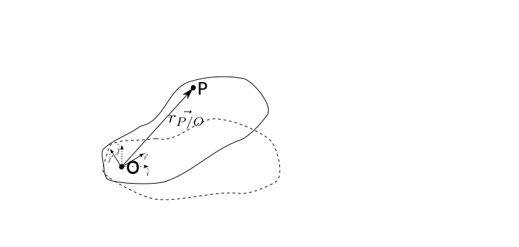
The description of the position of a point P of a rotating rigid body is given by:

\begin{equation} {\bf\vec{r}_{P/O}} = x_{P/O}^*{\bf\hat{i}'} + y_{P/O}^*{\bf\hat{j}'} \end{equation}

where $x_{P/O}^*$ and $y_{P/O}^*$ are the coordinates of the point P position at a reference state with the versors described as:

\begin{equation} {\bf\hat{i}'} = \cos(\theta){\bf\hat{i}}+\sin(\theta){\bf\hat{j}} \end{equation} \begin{equation} {\bf\hat{j}'} = -\sin(\theta){\bf\hat{i}}+\cos(\theta){\bf\hat{j}} \end{equation}

Note that the vector ${\bf\vec{r}_{P/O}}$ has always the same description for any point P of the rigid body when described as a linear combination of ${\bf\hat{i}'}$ and ${\bf\hat{j}'}$.

Translation of a rigid body

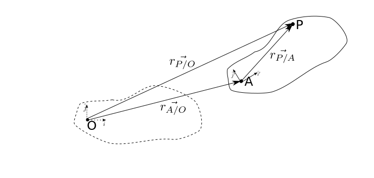
Let's consider now the case in which, besides a rotation, a translation of the body happens. This situation is represented in the figure below. In this case, the position of the point P is given by:

\begin{equation} {\bf\vec{r}_{P/O}} = {\bf\vec{r}_{A/O}}+{\bf\vec{r}_{P/A}}= {\bf\vec{r}_{A/O}}+x_{P/A}^*{\bf\hat{i}'} + y_{P/A}^*{\bf\hat{j}'} \end{equation}

Angular velocity of a body

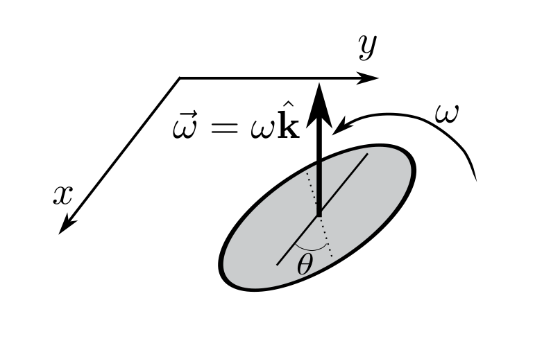
The magnitude of the angular velocity of a rigid body rotating on a plane is defined as:

\begin{equation} \omega = \frac{d\theta}{dt} \end{equation}

Usually, it is defined an angular velocity vector perpendicular to the plane where the rotation occurs (in this case the x-y plane) and with magnitude $\omega$:

\begin{equation} \vec{\bf{\omega}} = \omega\hat{\bf{k}} \end{equation}

Velocity of a point with no translation

First we will consider the situation with no translation. The velocity of the point P is given by:

\begin{equation} {\bf\vec{v}_{P/O}} = \frac{d{\bf\vec{r}_{P/O}}}{dt} = \frac{d(x_{P/O}^*{\bf\hat{i}'} + y_{P/O}^*{\bf\hat{j}'})}{dt} \end{equation}

To continue this deduction, we have to find the expression of the derivatives of ${\bf\hat{i}'}$ and ${\bf\hat{j}'}$. This is very similar to the derivative expressions of ${\bf\hat{e_R}}$ and ${\bf\hat{e_\theta}}$ of polar basis.

\begin{equation} \frac{d{\bf\hat{i}'}}{dt} = -\dot{\theta}\sin(\theta){\bf\hat{i}}+\dot{\theta}\cos(\theta){\bf\hat{j}} = \dot{\theta}{\bf\hat{j}'} \end{equation} \begin{equation} \frac{d{\bf\hat{j}'}}{dt} = -\dot{\theta}\cos(\theta){\bf\hat{i}}-\dot{\theta}\sin(\theta){\bf\hat{j}} = -\dot{\theta}{\bf\hat{i}'} \end{equation}

Another way to represent the expressions above is by using the vector form to express the angular velocity $\dot{\theta}$. It is usual to represent the angular velocity as a vector in the direction ${\bf\hat{k}}$: ${\bf\vec{\omega}} = \dot{\theta}{\bf\hat{k}} = \omega{\bf\hat{k}}$. Using this definition of the angular velocity, we can write the above expressions as:

\begin{equation} \frac{d{\bf\hat{i}'}}{dt} = \dot{\theta}{\bf\hat{j}'} = \dot{\theta} {\bf\hat{k}}\times {\bf\hat{i}'} = {\bf\vec{\omega}} \times {\bf\hat{i}'} \end{equation} \begin{equation} \frac{d{\bf\hat{j}'}}{dt} = -\dot{\theta}{\bf\hat{i}'} = \dot{\theta} {\bf\hat{k}}\times {\bf\hat{j}'} ={\bf\vec{\omega}} \times {\bf\hat{j}'} \end{equation}

So, the velocity of the point P in the situation of no translation is:

\begin{equation} {\bf\vec{v}_{P/O}} = \frac{d(x_{P/O}^*{\bf\hat{i}'} + y_{P/O}^*{\bf\hat{j}'})}{dt} = x_{P/O}^*\frac{d{\bf\hat{i}'}}{dt} + y_{P/O}^*\frac{d{\bf\hat{j}'}}{dt}=x_{P/O}^*{\bf\vec{\omega}} \times {\bf\hat{i}'} + y_{P/O}^*{\bf\vec{\omega}} \times {\bf\hat{j}'} = {\bf\vec{\omega}} \times \left(x_{P/O}^*{\bf\hat{i}'}\right) + {\bf\vec{\omega}} \times \left(y_{P/O}^*{\bf\hat{j}'}\right) ={\bf\vec{\omega}} \times \left(x_{P/O}^*{\bf\hat{i}'}+y_{P/O}^*{\bf\hat{j}'}\right) \end{equation} \begin{equation} {\bf\vec{v}_{P/O}} = {\bf\vec{\omega}} \times {\bf{\vec{r}_{P/O}}} \end{equation}

This expression shows that the velocity vector of any point of a rigid body is orthogonal to the vector linking the point O and the point P.

It is worth to note that despite the above expression was deduced for a planar movement, the expression above is general, including three dimensional movements.

Relative velocity of a point on a rigid body to another point

To compute the velocity of a point on a rigid body that is translating, we need to find the expression of the velocity of a point (P) in relation to another point on the body (A). So:

\begin{equation} {\bf\vec{v}_{P/A}} = {\bf\vec{v}_{P/O}}-{\bf\vec{v}_{A/O}} = {\bf\vec{\omega}} \times {\bf{\vec{r}_{P/O}}} - {\bf\vec{\omega}} \times {\bf{\vec{r}_{A/O}}} = {\bf\vec{\omega}} \times ({\bf{\vec{r}_{P/O}}}-{\bf{\vec{r}_{A/O}}}) = {\bf\vec{\omega}} \times {\bf{\vec{r}_{P/A}}} \end{equation}

Velocity of a point on rigid body translating

The velocity of a point on a rigid body that is translating is given by:

\begin{equation} {\bf\vec{v}_{P/O}} = \frac{d{\bf\vec{r}_{P/O}}}{dt} = \frac{d({\bf\vec{r}_{A/O}}+x_{P/A}^*{\bf\hat{i}'} + y_{P/A}^*{\bf\hat{j}'})}{dt} = \frac{d{\bf\vec{r}_{A/O}}}{dt}+\frac{d(x_{P/A}^*{\bf\hat{i}'} + y_{P/A}^*{\bf\hat{j}'})}{dt} = {\bf\vec{v}_{A/O}} + {\bf\vec{\omega}} \times {\bf{\vec{r}_{P/A}}} \end{equation}

Below is an example of a body rotating with the angular velocity of $\omega = \pi/10$ rad/s and translating at the velocity of ${\bf\vec{v}} = 0.7 {\bf\hat{i}} + 0.5 {\bf\hat{j}}$ m/s. The red arrow indicates the velocity of the geometric center of the body and the blue arrow indicates the velocity of the lower point of the body

t = np.linspace(0,13,40)
omega = np.pi/10 #[rad/s] 
voa = np.array([[0.7],[0.5]]) # velocity of center of mass
fig = plt.figure()
plt.grid()
ax = fig.add_axes([0, 0, 1, 1])    
ax.axis("on")
plt.rcParams['figure.figsize']=5,5
def run(i):
    ax.clear()
    theta = omega * t[i]
    phi = np.linspace(0,2*np.pi,100)
    B = np.squeeze(np.array([[2*np.cos(phi)],[6*np.sin(phi)]]))
    Baum = np.vstack((B,np.ones((1,np.shape(B)[1]))))
    roa = voa * t[i]
    R = np.array([[np.cos(theta), -np.sin(theta)],[np.sin(theta), np.cos(theta)]])
    T = np.vstack((np.hstack((R,roa)), np.array([0,0,1])))
    BRot = R@B
    BRotTr = T@Baum   
    
    
    
    plt.plot(BRotTr[0,:],BRotTr[1,:], roa[0], roa[1],'.')
    plt.fill(BRotTr[0,:],BRotTr[1,:], 'g')
    
    vVoa = FancyArrowPatch(roa.squeeze(), roa.squeeze()+5*voa.squeeze(), mutation_scale=20, 
                           lw=2, arrowstyle="->", color="r", alpha=1)
    ax.add_artist(vVoa)   
    
    element = 75
    
    # cross product between omega and r
    Vp = voa + np.cross(np.array([0,0,omega]), BRot[:,[element]].T)[:,0:2].T 
   
    vVP = FancyArrowPatch(BRotTr[0:2,element], BRotTr[0:2,element] + 5*Vp.squeeze(),
                          mutation_scale=20, 
                          lw=2, arrowstyle="->", color="b", alpha=1)
    ax.add_artist(vVP)
    
    plt.xlim((-10, 20))
    plt.ylim((-10, 20))
     
ani = FuncAnimation(fig, run, frames = 50, repeat=False,  interval =500)
plt.show()

Figure

Acceleration of a point on a rigid body

The acceleration of a point on a rigid body is obtained by deriving the previous expression:

\begin{align} {\bf\vec{a}_{P/O}} =& {\bf\vec{a}_{A/O}} + \dot{\bf\vec{\omega}} \times {\bf{\vec{r}_{P/A}}} + {\bf\vec{\omega}} \times {\bf{\vec{v}_{P/A}}} =\\ =&{\bf\vec{a}_{A/O}} + \dot{\bf\vec{\omega}} \times {\bf{\vec{r}_{P/A}}} + {\bf\vec{\omega}} \times ({\bf\vec{\omega}} \times {\bf{\vec{r}_{P/A}}}) =\\ =&{\bf\vec{a}_{A/O}} + \ddot{\theta}\bf\hat{k} \times {\bf{\vec{r}_{P/A}}} - \dot{\theta}^2{\bf{\vec{r}_{P/A}}} \end{align}

The acceleration has three terms:

• ${\bf\vec{a}_{A/O}}$ -- the acceleration of the point O.
• $\ddot{\theta}\bf\hat{k} \times {\bf{\vec{r}_{P/A}}}$ -- the acceleration of the point P due to the angular acceleration of the body.
• $- \dot{\theta}^2{\bf{\vec{r}_{P/A}}}$ -- the acceleration of the point P due to the angular velocity of the body. It is known as centripetal acceleration.

Below is an example of a rigid body with an angular acceleration of $\alpha = \pi/150$ rad/s$^2$ and initial angular velocity of $\omega_0 = \pi/100$ rad/s. Consider also that the center of the body accelerates with ${\bf\vec{a}} = 0.01{\bf\hat{i}} + 0.05{\bf\hat{j}}$, starting from rest.

t = np.linspace(0, 20, 40)

alpha = np.pi/150 #[rad/s^2] angular acceleration 

omega0 = np.pi/100 #[rad/s] angular velocity

aoa = np.array([[0.01],[0.05]]) # linear acceleration

fig = plt.figure()
plt.grid()
ax = fig.add_axes([0, 0, 1, 1])    
ax.axis("on")
plt.rcParams['figure.figsize']=5,5
theta = 0
omega = 0
def run(i):
    ax.clear()
    phi = np.linspace(0,2*np.pi,100)
    B = np.squeeze(np.array([[2*np.cos(phi)],[6*np.sin(phi)]]))
    Baum = np.vstack((B,np.ones((1,np.shape(B)[1]))))
    
    omega = alpha*t[i]+omega0 #[rad/s] angular velocity
    
    theta = alpha/2*t[i]**2 + omega0*t[i] # [rad] angle
    
    voa = aoa*t[i] # linear velocity
    
    roa = aoa/2*t[i]**2 # position of the center of the body
    
    R = np.array([[np.cos(theta), -np.sin(theta)],[np.sin(theta), np.cos(theta)]])
    T = np.vstack((np.hstack((R,roa)), np.array([0,0,1])))
    BRot = R@B
    BRotTr = T@Baum   
    
    plt.plot(BRotTr[0,:],BRotTr[1,:], roa[0], roa[1],'.')
    plt.fill(BRotTr[0,:],BRotTr[1,:],'g')
    
    element = 75
   
    ap = (aoa + np.cross(np.array([0,0,alpha]), BRot[:,[element]].T)[:,0:2].T  
          - omega**2*BRot[:,[element]])
    
    vVP = FancyArrowPatch(BRotTr[0:2,element], BRotTr[0:2,element] + 5*ap.squeeze(),
                          mutation_scale=20, 
                          lw=2, arrowstyle="->", color="b", alpha=1)
    ax.add_artist(vVP)
    
    plt.xlim((-10, 20))
    plt.ylim((-10, 20))
       
    

ani = FuncAnimation(fig, run, frames=50, repeat=False,  interval=500)
plt.show()

Figure

Further reading

• Read pages 958-971 of the 18th chapter of the [Ruina and Rudra's book] (http://ruina.tam.cornell.edu/Book/index.html) about circular motion of particle.

Video lectures on the Internet

• Kinematics Of Rigid Bodies - General Plane Motion - Solved Problems
• Kinematics of Rigid Bodies -Translation And Rotation About Fixed Axis - Rectilinear and Rotational

Problems

• 1. Solve the problems 16.2.5, 16.2.10, 16.2.11 and 16.2.20 from Ruina and Rudra's book.
• 2. Solve the problems 17.1.2, 17.1.8, 17.1.9, 17.1.10, 17.1.11 and 17.1.12 from Ruina and Rudra's book.
• 3. Solve the problems 2.1, 2.2, 2.7, 2.8, 2.17

Reference

• Ruina A, Rudra P (2019) Introduction to Statics and Dynamics. Oxford University Press.
• Corke P (2017) Robotics, Vision and Control: Fundamental Algorithms in MATLAB. 2nd ed. Springer-Verlag Berlin.