Papers / Sites
- Comparsion of Tracking Methods in Biology
- Chenouard, N., Smal, I., de Chaumont, F., Maška, M., Sbalzarini, I. F., Gong, Y., … Meijering, E. (2014). Objective comparison of particle tracking methods. Nature Methods, 11(3), 281–289. doi:10.1038/nmeth.2808
- Maska, M., Ulman, V., Svoboda, D., Matula, P., Matula, P., Ederra, C., … Ortiz-de-Solorzano, C. (2014). A benchmark for comparison of cell tracking algorithms. Bioinformatics (Oxford, England), btu080–. doi:10.1093/bioinformatics/btu080
- Keypoint and Corner Detection
- Distinctive Image Features from Scale-Invariant Keypoints - https://www.cs.ubc.ca/~lowe/papers/ijcv04.pdf
- https://opencv-python-tutroals.readthedocs.io/en/latest/py_tutorials/py_feature2d/py_sift_intro/py_sift_intro.html
- Registration
- https://itk.org/ITKSoftwareGuide/html/Book2/ITKSoftwareGuide-Book2ch3.html
- Multiple Hypothesis Testing
- Coraluppi, S. & Carthel, C. Multi-stage multiple-hypothesis tracking.
J. Adv. Inf. Fusion 6, 57–67 (2011).
- Chenouard, N., Bloch, I. & Olivo-Marin, J.-C. Multiple hypothesis
tracking in microscopy images. in Proc. IEEE Int. Symp. Biomed. Imaging 1346–1349 (IEEE, 2009).
Previously on QBI ...
- Image Enhancment
- Highlighting the contrast of interest in images
- Minimizing Noise
- Understanding image histograms
- Automatic Methods
- Component Labeling
- Single Shape Analysis
- Complicated Shapes
- Distribution Analysis
Quantitative "Big" Imaging
The course has covered imaging enough and there have been a few quantitative metrics, but "big" has not really entered.
What does big mean?
- Not just / even large
- it means being ready for big data
- The three V's
- volume,
- velocity,
- variety
- scalable, fast, easy to customize
So what is "big" imaging
- doing analyses in a disciplined manner
- fixed steps
- easy to regenerate results
- no magic
- having everything automated
- 100 samples is as easy as 1 sample
- being able to adapt and reuse analyses
- one really well working script and modify parameters
- different types of cells
- different regions
Objectives
Experiments
- What sort of dynamic experiments do we have?
- How can we design good dynamic experiments?
Image analysis
- How can we track objects between points?
- How can we track shape?
- How can we track distribution?
- How can we track topology?
- How can we track voxels?
- How can we assess deformation and strain?
- How can assess more general cases?
$\rightarrow$ How does this help answering your questions?
Motivation
- 3D images are already difficult to interpret on their own
- 3D movies (4D) are almost impossible

What information are you looking for?
We can say that it looks like, but many pieces of quantitative information are difficult to extract
- How fast is it going?
- How many particles are present?
- Are their sizes constant?
- Are some moving faster?
- Are they rearranging?
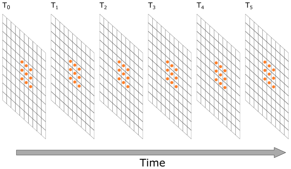
Stage Tilting
Beyond just tracking we can take multiple frames of a still image and instead of looking for changes in the object, we can change the angle. The pollen image below shows this for SEM
Scientific Goals of dynamic experiments
Rheology
Understanding the flow of liquids and mixtures is important for many processes
- blood movement in arteries, veins, and capillaries
- oil movement through porous rock
- air through dough when cooking bread
- magma and gas in a volcano
Deformation
Deformation is similarly important since it plays a significant role in the following scenarios
- red blood cell lysis in artificial heart valves
- microfractures growing into stress fractures in bone
- toughening in certain wood types
Experiments
The first step of any of these analyses is proper experimental design. Since there is always:
- A limited field of view
- A voxel size
- A maximum rate of measurements
- Dose limitations
- Sample damage
- Limited flux
- A non-zero cost for each measurement
There are always trade-offs to be made between getting the best possible high-resolution nanoscale dynamics and capturing the system level behavior.
Planning dynamic experiments
If we measure too fast
Too slow
Too high resolution
Too low resolution
|

|
Tuning experiment by simulation
In many cases:
- experimental data is inherited
- little can be done about the design,
When there is still the opportunity to tune the experiment
simulations provide a powerful tool for tuning and balancing a large number parameters
Validation
Simulations also provide the ability to pair post-processing to the experiments and determine the limits of tracking.
What do we start with?
Going back to our original cell image
- We have been able to get rid of the noise in the image and find all the cells (lecture 2-4)
- We have analyzed the shape of the cells using the shape tensor (lecture 5)
- We even separated cells joined together using Watershed (lecture 6)
- We have created even more metrics characterizing the distribution (lecture 7)
We have at least a few samples (or different regions), large number of metrics and an almost as large number of parameters to tune
How do we do something meaningful with it?
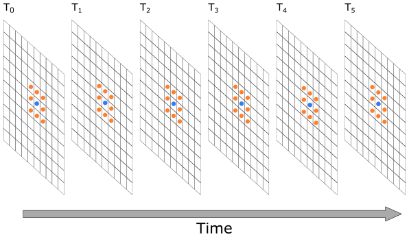
Basic Simulation
We start with a starting image with a number of circles on a plane
import numpy as np
import matplotlib.pyplot as plt
from skimage.io import imread
%matplotlib inline
xx, yy = np.meshgrid(np.linspace(-1.5, 1.5, 15),
np.linspace(-1.5, 1.5, 15))
N_DISK_ROW = 2
N_DISK_COL = 4
DISK_RAD = 0.15
disk_img = np.zeros(xx.shape, dtype=int)
for x_cent in 0.7*np.linspace(-1, 1, N_DISK_COL):
for y_cent in 0.7*np.linspace(-1, 1, N_DISK_ROW):
c_disk = np.sqrt(np.square(xx-x_cent)+np.square(yy-y_cent)) < DISK_RAD
disk_img[c_disk] = 1
fig, ax1 = plt.subplots(1, 1)
sns.heatmap(disk_img, annot=True, fmt='d', ax=ax1);

Create a series of moving "cells"
from matplotlib.animation import FuncAnimation
from IPython.display import HTML
fig, c_ax = plt.subplots(1, 1, figsize=(5, 5), dpi=100)
s_img = disk_img.copy()
img_list = [s_img]
for i in range(4):
s_img = np.roll(s_img, -1, axis=1)
s_img = np.roll(s_img, -1, axis=0)
img_list += [s_img]
def update_frame(i):
plt.cla()
sns.heatmap(img_list[i],annot=True,
fmt="d",cmap='nipy_spectral',
ax=c_ax,cbar=False,
vmin=0,vmax=1)
c_ax.set_title('Iteration #{}'.format(i+1))
# write animation frames
anim_code = FuncAnimation(fig,
update_frame,
frames=len(img_list),
interval=1000, repeat_delay=2000).to_html5_video()
plt.close('all')
HTML(anim_code)
Analysis
The analysis of the series requires the following steps:
- Threshold
- Component Label
- Shape Analysis
- Distribution Analysis
... and to put all in a data frame
from skimage.morphology import label
from skimage.measure import regionprops
import pandas as pd
all_objs = []
for frame_idx, c_img in enumerate(img_list): # For each time frame
lab_img = label(c_img > 0) # Label
for c_obj in regionprops(lab_img): # Put region properties for each object of the time frame
all_objs += [dict(label=int(c_obj.label),
y=c_obj.centroid[0],
x=c_obj.centroid[1],
area=c_obj.area,
frame_idx=frame_idx)]
all_obj_df = pd.DataFrame(all_objs) # Create a Pandas data frame with all the properties
all_obj_df.head(5) # Look at the first five rows of the data frame
| label | y | x | area | frame_idx | |
|---|---|---|---|---|---|
| 0 | 1 | 4.0 | 4.0 | 1 | 0 |
| 1 | 2 | 4.0 | 6.0 | 1 | 0 |
| 2 | 3 | 4.0 | 8.0 | 1 | 0 |
| 3 | 4 | 4.0 | 10.0 | 1 | 0 |
| 4 | 5 | 10.0 | 4.0 | 1 | 0 |
Looking at the positions of the items in all frames
fig, c_ax = plt.subplots(1, 1, figsize=(5, 5), dpi=150)
c_ax.imshow(disk_img, cmap='bone_r')
for frame_idx, c_rows in all_obj_df.groupby('frame_idx'):
c_ax.plot(c_rows['x'], c_rows['y'], 's', label='Frame: %d' % frame_idx)
c_ax.legend();

Describing Motion
We can describe the motion in the above example with a simple vector
$$ \vec{v}(\vec{x})=\langle -1,-1 \rangle $$Scoring Tracking
In the following examples we will use simple metrics for scoring fits where the objects are matched and the number of misses is counted.
There are a number of more sensitive scoring metrics which can be used, by finding the best submatch for a given particle since the number of matches and particles does not always correspond.
See the papers at the beginning for more information
Tracking methods
While there exist a number of different methods and complicated approaches for tracking.
For experimental design it is best to start with the
- simplest
- easiest understood
method.
The limits of this can be found and components added as needed until it is possible to realize the experiment
If a dataset can only be analyzed with a multiple-hypothesis testing neural network model then it might not be so reliable
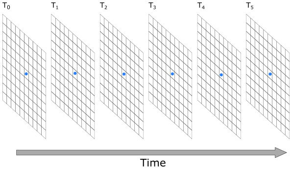
Tracking using Nearest Neighbor
We then return to nearest neighbor which means we track
- a point ($\vec{P}_0$) from an image ($I_0$) at $t_0$
- to a point ($\vec{P}_1$) in image ($I_1$) at $t_1$
by
$$ \vec{P}_1=\textrm{argmin}(||\vec{P}_0-\vec{y}|| \;\forall \vec{y}\in I_1) $$Distances between objects
frame_0 = all_obj_df[all_obj_df['frame_idx'].isin([0])]
frame_1 = all_obj_df[all_obj_df['frame_idx'].isin([1])]
fig, c_ax = plt.subplots(1, 1, figsize=(5, 5), dpi=150)
c_ax.matshow(1 < disk_img , cmap='gist_yarg')
c_ax.scatter(frame_0['x'], frame_0['y'], c='black', label='Frame: 0')
c_ax.scatter(frame_1['x'], frame_1['y'], c='red', label='Frame: 1')
dist_df_list = []
for _, row_0 in frame_0.iterrows():
for _, row_1 in frame_1.iterrows():
seg_dist = np.sqrt(np.square(row_0['x']-row_1['x']) +
np.square(row_0['y']-row_1['y']))
c_ax.plot([row_0['x'], row_1['x']],
[row_0['y'], row_1['y']], '-', alpha=1/seg_dist)
dist_df_list += [dict(x0=row_0['x'],
y0=row_0['y'],
lab0=int(row_0['label']),
x1=row_1['x'],
y1=row_1['y'],
lab1=int(row_1['label']),
dist=seg_dist)]
c_ax.legend();

Put the distances in a data frame
dist_df = pd.DataFrame(dist_df_list)
dist_df.head(5)
| x0 | y0 | lab0 | x1 | y1 | lab1 | dist | |
|---|---|---|---|---|---|---|---|
| 0 | 4.0 | 4.0 | 1 | 3.0 | 3.0 | 1 | 1.414214 |
| 1 | 4.0 | 4.0 | 1 | 5.0 | 3.0 | 2 | 1.414214 |
| 2 | 4.0 | 4.0 | 1 | 7.0 | 3.0 | 3 | 3.162278 |
| 3 | 4.0 | 4.0 | 1 | 9.0 | 3.0 | 4 | 5.099020 |
| 4 | 4.0 | 4.0 | 1 | 3.0 | 9.0 | 5 | 5.099020 |
from matplotlib.animation import FuncAnimation
from IPython.display import HTML
fig, c_ax = plt.subplots(1, 1, figsize=(5, 5), dpi=150)
c_ax.matshow(disk_img > 1, cmap='gist_yarg')
c_ax.scatter(frame_0['x'], frame_0['y'], c='black', label='Frame: 0')
c_ax.scatter(frame_1['x'], frame_1['y'], c='red', label='Frame: 1')
def update_frame(i):
# plt.cla()
c_rows = dist_df.query('lab0==%d' % i)
for _, c_row in c_rows.iterrows():
c_ax.quiver(c_row['x0'], c_row['y0'],
c_row['x1']-c_row['x0'],
c_row['y1']-c_row['y0'], scale=1.0, scale_units='xy', angles='xy',
alpha=1/c_row['dist'])
c_ax.set_title('Point #{}'.format(i+1))
# write animation frames
anim_code = FuncAnimation(fig,
update_frame,
frames=np.unique(dist_df['lab0']),
interval=1000,
repeat_delay=2000).to_html5_video()
plt.close('all')
HTML(anim_code)
fig, c_ax = plt.subplots(1, 1, figsize=(5, 5), dpi=150)
c_ax.matshow(disk_img > 1,cmap='gist_yarg')
c_ax.scatter(frame_0['x'], frame_0['y'], c='black', label='Frame: 0')
c_ax.scatter(frame_1['x'], frame_1['y'], c='red', label='Frame: 1')
for _, c_rows in dist_df.groupby('lab0'):
_, c_row = next(c_rows.sort_values('dist').iterrows())
c_ax.quiver(c_row['x0'], c_row['y0'],
c_row['x1']-c_row['x0'],
c_row['y1']-c_row['y0'],
scale=1.0, scale_units='xy', angles='xy')
c_ax.legend();

from matplotlib.animation import FuncAnimation
from IPython.display import HTML
fig, c_ax = plt.subplots(1, 1, figsize=(5, 5), dpi=150)
c_ax.matshow(disk_img > 1,cmap='gist_yarg')
def draw_timestep(i):
# plt.cla()
frame_0 = all_obj_df[all_obj_df['frame_idx'].isin([i])]
frame_1 = all_obj_df[all_obj_df['frame_idx'].isin([i+1])]
c_ax.scatter(frame_0['x'], frame_0['y'], c='black', label='Frame: %d' % i)
c_ax.scatter(frame_1['x'], frame_1['y'],
c='red', label='Frame: %d' % (i+1))
dist_df_list = []
for _, row_0 in frame_0.iterrows():
for _, row_1 in frame_1.iterrows():
dist_df_list += [dict(x0=row_0['x'],
y0=row_0['y'],
lab0=int(row_0['label']),
x1=row_1['x'],
y1=row_1['y'],
lab1=int(row_1['label']),
dist=np.sqrt(
np.square(row_0['x']-row_1['x']) +
np.square(row_0['y']-row_1['y'])))]
dist_df = pd.DataFrame(dist_df_list)
for _, c_rows in dist_df.groupby('lab0'):
_, best_row = next(c_rows.sort_values('dist').iterrows())
c_ax.quiver(best_row['x0'], best_row['y0'],
best_row['x1']-best_row['x0'],
best_row['y1']-best_row['y0'],
scale=1.0, scale_units='xy', angles='xy')
c_ax.set_title('Frame #{}'.format(i+1))
# write animation frames
anim_code = FuncAnimation(fig,
draw_timestep,
frames=all_obj_df['frame_idx'].max(),
interval=1000,
repeat_delay=2000).to_html5_video()
plt.close('all')
HTML(anim_code)
Computing Average Flow
From each of these time steps we can now proceed to compute the average flow.
We can perform this :
- spatially (averaging over regions and time),
- temporally (averaging over regions),
- or spatial-temporally (averaging over regions for every time step)
average_field = []
for i in range(all_obj_df['frame_idx'].max()):
frame_0 = all_obj_df[all_obj_df['frame_idx'].isin([i])]
frame_1 = all_obj_df[all_obj_df['frame_idx'].isin([i+1])]
dist_df_list = []
for _, row_0 in frame_0.iterrows():
for _, row_1 in frame_1.iterrows():
dist_df_list += [dict(x0=row_0['x'],
y0=row_0['y'],
lab0=int(row_0['label']),
x1=row_1['x'],
y1=row_1['y'],
lab1=int(row_1['label']),
dist=np.sqrt(
np.square(row_0['x']-row_1['x']) +
np.square(row_0['y']-row_1['y'])))]
dist_df = pd.DataFrame(dist_df_list)
for _, c_rows in dist_df.groupby('lab0'):
_, best_row = next(c_rows.sort_values('dist').iterrows())
average_field += [dict(frame_idx=i,
x=best_row['x0'],
y=best_row['y0'],
dx=best_row['x1']-best_row['x0'],
dy=best_row['y1']-best_row['y0'])]
average_field_df = pd.DataFrame(average_field)
print('Average Flow:')
average_field_df[['dx', 'dy']].mean()
Average Flow:
dx -1.0 dy -1.0 dtype: float64
Spatially Averaging
To spatially average we first create a grid of values and then interpolate our results onto this grid
from scipy.interpolate import interp2d
def img_intp(f):
def new_f(x, y):
return np.stack([f(ix, iy) for ix, iy in zip(np.ravel(x), np.ravel(y))], 0).reshape(np.shape(x))
return new_f
dx_func = img_intp(
interp2d(average_field_df['x'], average_field_df['y'], average_field_df['dx']))
dy_func = img_intp(
interp2d(average_field_df['x'], average_field_df['y'], average_field_df['dy']))
dx_func(8, 8), dy_func(8, 8)
C:\Users\ander\anaconda3\lib\site-packages\scipy\interpolate\_fitpack_impl.py:976: RuntimeWarning: No more knots can be added because the number of B-spline coefficients already exceeds the number of data points m. Probable causes: either s or m too small. (fp>s) kx,ky=1,1 nx,ny=7,9 m=32 fp=0.000000 s=0.000000 warnings.warn(RuntimeWarning(_iermess2[ierm][0] + _mess))
(array(-1.), array(-1.))
g_x, g_y = np.meshgrid(np.linspace(average_field_df['x'].min(),
average_field_df['x'].max(), 10),
np.linspace(average_field_df['y'].min(),
average_field_df['y'].max(), 10))
fig, (ax1, ax2, ax3, ax4, ax5) = plt.subplots(1, 5, figsize=(24, 4))
sns.heatmap(g_x, ax=ax1, annot=True)
ax1.set_title('X Position')
sns.heatmap(g_y, ax=ax2, annot=True)
ax2.set_title('Y Position')
sns.heatmap(dx_func(g_x, g_y), ax=ax3, annot=True)
ax3.set_title('$\Delta x$')
sns.heatmap(dy_func(g_x, g_y), ax=ax4, annot=True)
ax4.set_title('$\Delta y$')
ax5.quiver(g_x, g_y, dx_func(g_x, g_y), dy_func(g_x, g_y),
scale=1.0, scale_units='xy', angles='xy');

Temporarly Averaging
Here we take the average at each time point
temp_avg_field = average_field_df[['frame_idx', 'dx', 'dy']].groupby(
'frame_idx').agg('mean').reset_index()
temp_avg_field
| frame_idx | dx | dy | |
|---|---|---|---|
| 0 | 0 | -1.0 | -1.0 |
| 1 | 1 | -1.0 | -1.0 |
| 2 | 2 | -1.0 | -1.0 |
| 3 | 3 | -1.0 | -1.0 |
fig, (ax1, ax2, ax3) = plt.subplots(1, 3, figsize=(18, 4))
ax1.plot(temp_avg_field['frame_idx'], temp_avg_field['dx'], 'rs-')
ax1.set_title('$\Delta x$')
ax1.set_xlabel('Timestep')
ax2.plot(temp_avg_field['frame_idx'], temp_avg_field['dy'], 'rs-')
ax2.set_title('$\Delta y$')
ax2.set_xlabel('Timestep')
ax3.quiver(temp_avg_field['dx'], temp_avg_field['dy'],
scale=1, scale_units='xy', angles='xy')
ax3.set_title('$\Delta x$, $\Delta y$')
ax3.set_xlabel('Timestep')
Text(0.5, 0, 'Timestep')

Spatiotemporal Relationship
We can also divide the images into space and time steps
from matplotlib.animation import FuncAnimation
from IPython.display import HTML
g_x, g_y = np.meshgrid(np.linspace(average_field_df['x'].min(),
average_field_df['x'].max(), 4),
np.linspace(average_field_df['y'].min(),
average_field_df['y'].max(), 4))
frames = len(sorted(np.unique(average_field_df['frame_idx'])))
fig, m_axs = plt.subplots(2, 3, figsize=(14, 10))
for c_ax in m_axs.flatten():
c_ax.axis('off')
[(ax1, ax2, _), (ax3, ax4, ax5)] = m_axs
def draw_frame_idx(idx):
plt.cla()
c_df = average_field_df[average_field_df['frame_idx'].isin([idx])]
dx_func = img_intp(interp2d(c_df['x'], c_df['y'], c_df['dx']))
dy_func = img_intp(interp2d(c_df['x'], c_df['y'], c_df['dy']))
sns.heatmap(g_x, ax=ax1, annot=False, cbar=False)
ax1.set_title('Frame %d\nX Position' % idx)
sns.heatmap(g_y, ax=ax2, annot=False, cbar=False)
ax2.set_title('Y Position')
sns.heatmap(dx_func(g_x, g_y), ax=ax3, annot=False, cbar=False, fmt='2.1f')
ax3.set_title('$\Delta x$')
sns.heatmap(dy_func(g_x, g_y), ax=ax4, annot=False, cbar=False, fmt='2.1f')
ax4.set_title('$\Delta y$')
ax5.quiver(g_x, g_y, dx_func(g_x, g_y), dy_func(g_x, g_y),
scale=1.0, scale_units='xy', angles='xy')
# write animation frames
anim_code = FuncAnimation(fig,
draw_frame_idx,
frames=frames,
interval=1000,
repeat_delay=2000).to_html5_video()
plt.close('all')
HTML(anim_code)
C:\Users\ander\anaconda3\lib\site-packages\scipy\interpolate\_fitpack_impl.py:976: RuntimeWarning: No more knots can be added because the number of B-spline coefficients already exceeds the number of data points m. Probable causes: either s or m too small. (fp>s) kx,ky=1,1 nx,ny=5,5 m=8 fp=0.000000 s=0.000000 warnings.warn(RuntimeWarning(_iermess2[ierm][0] + _mess))
Longer Series
We see that this approach becomes problematic when we want to work with longer series
import pandas as pd
from skimage.morphology import label
from skimage.measure import regionprops
from matplotlib.animation import FuncAnimation
from IPython.display import HTML
fig, c_ax = plt.subplots(1, 1, figsize=(5, 5), dpi=150)
s_img = disk_img.copy()
img_list = [s_img]
for i in range(8):
if i % 2 == 0:
s_img = np.roll(s_img, -2, axis=0)
else:
s_img = np.roll(s_img, -1, axis=1)
img_list += [s_img]
all_objs = []
for frame_idx, c_img in enumerate(img_list):
lab_img = label(c_img > 0)
for c_obj in regionprops(lab_img):
all_objs += [dict(label=int(c_obj.label),
y=c_obj.centroid[0],
x=c_obj.centroid[1],
area=c_obj.area,
frame_idx=frame_idx)]
all_obj_df = pd.DataFrame(all_objs)
all_obj_df.head(5)
def update_frame(i):
plt.cla()
sns.heatmap(img_list[i],
annot=True,
fmt="d",
cmap='nipy_spectral',
ax=c_ax,
cbar=False,
vmin=0,
vmax=1)
c_ax.set_title('Iteration #{}'.format(i+1))
# write animation frames
anim_code = FuncAnimation(fig,
update_frame,
frames=len(img_list),
interval=1000,
repeat_delay=2000).to_html5_video()
plt.close('all')
HTML(anim_code)
from matplotlib.animation import FuncAnimation
from IPython.display import HTML
fig, c_ax = plt.subplots(1, 1, figsize=(5, 5), dpi=150)
c_ax.matshow(disk_img > 1,cmap='gist_yarg')
def draw_timestep(i):
# plt.cla()
frame_0 = all_obj_df[all_obj_df['frame_idx'].isin([i])]
frame_1 = all_obj_df[all_obj_df['frame_idx'].isin([i+1])]
c_ax.scatter(frame_0['x'], frame_0['y'], c='black', label='Frame: %d' % i)
c_ax.scatter(frame_1['x'], frame_1['y'],
c='red', label='Frame: %d' % (i+1))
dist_df_list = []
for _, row_0 in frame_0.iterrows():
for _, row_1 in frame_1.iterrows():
dist_df_list += [dict(x0=row_0['x'],
y0=row_0['y'],
lab0=int(row_0['label']),
x1=row_1['x'],
y1=row_1['y'],
lab1=int(row_1['label']),
dist=np.sqrt(
np.square(row_0['x']-row_1['x']) +
np.square(row_0['y']-row_1['y'])))]
dist_df = pd.DataFrame(dist_df_list)
for _, c_rows in dist_df.groupby('lab0'):
_, best_row = next(c_rows.sort_values('dist').iterrows())
c_ax.quiver(best_row['x0'], best_row['y0'],
best_row['x1']-best_row['x0'],
best_row['y1']-best_row['y0'],
scale=1.0, scale_units='xy', angles='xy', alpha=0.25)
c_ax.set_title('Frame #{}'.format(i+1))
# write animation frames
anim_code = FuncAnimation(fig,
draw_timestep,
frames=all_obj_df['frame_idx'].max(),
interval=1000,
repeat_delay=2000).to_html5_video()
plt.close('all')
HTML(anim_code)
from scipy.interpolate import interp2d
average_field = []
for i in range(all_obj_df['frame_idx'].max()):
frame_0 = all_obj_df[all_obj_df['frame_idx'].isin([i])]
frame_1 = all_obj_df[all_obj_df['frame_idx'].isin([i+1])]
dist_df_list = []
for _, row_0 in frame_0.iterrows():
for _, row_1 in frame_1.iterrows():
dist_df_list += [dict(x0=row_0['x'],
y0=row_0['y'],
lab0=int(row_0['label']),
x1=row_1['x'],
y1=row_1['y'],
lab1=int(row_1['label']),
dist=np.sqrt(
np.square(row_0['x']-row_1['x']) +
np.square(row_0['y']-row_1['y'])))]
dist_df = pd.DataFrame(dist_df_list)
for _, c_rows in dist_df.groupby('lab0'):
_, best_row = next(c_rows.sort_values('dist').iterrows())
average_field += [dict(frame_idx=i,
x=best_row['x0'],
y=best_row['y0'],
dx=best_row['x1']-best_row['x0'],
dy=best_row['y1']-best_row['y0'])]
average_field_df = pd.DataFrame(average_field)
print('Average Flow:')
print(average_field_df[['dx', 'dy']].mean())
def img_intp(f):
def new_f(x, y):
return np.stack([f(ix, iy) for ix, iy in zip(np.ravel(x), np.ravel(y))], 0).reshape(np.shape(x))
return new_f
dx_func = img_intp(
interp2d(average_field_df['x'], average_field_df['y'], average_field_df['dx']))
dy_func = img_intp(
interp2d(average_field_df['x'], average_field_df['y'], average_field_df['dy']))
g_x, g_y = np.meshgrid(np.linspace(average_field_df['x'].min(),
average_field_df['x'].max(), 5),
np.linspace(average_field_df['y'].min(),
average_field_df['y'].max(), 5))
fig, (ax1, ax2, ax3, ax4, ax5) = plt.subplots(1, 5, figsize=(24, 4))
sns.heatmap(g_x, ax=ax1, annot=True)
ax1.set_title('X Position')
sns.heatmap(g_y, ax=ax2, annot=True)
ax2.set_title('Y Position')
sns.heatmap(dx_func(g_x, g_y), ax=ax3, annot=True)
ax3.set_title('$\Delta x$')
sns.heatmap(dy_func(g_x, g_y), ax=ax4, annot=True)
ax4.set_title('$\Delta y$')
ax5.quiver(g_x, g_y, dx_func(g_x, g_y), dy_func(g_x, g_y),
scale=1.0, scale_units='xy', angles='xy');
Average Flow: dx -0.500 dy -0.625 dtype: float64
C:\Users\ander\anaconda3\lib\site-packages\scipy\interpolate\_fitpack_impl.py:976: RuntimeWarning: No more knots can be added because the number of B-spline coefficients already exceeds the number of data points m. Probable causes: either s or m too small. (fp>s) kx,ky=1,1 nx,ny=10,11 m=64 fp=5.301937 s=0.000000 warnings.warn(RuntimeWarning(_iermess2[ierm][0] + _mess)) C:\Users\ander\anaconda3\lib\site-packages\scipy\interpolate\_fitpack_impl.py:976: RuntimeWarning: No more knots can be added because the number of B-spline coefficients already exceeds the number of data points m. Probable causes: either s or m too small. (fp>s) kx,ky=1,1 nx,ny=10,11 m=64 fp=22.666667 s=0.000000 warnings.warn(RuntimeWarning(_iermess2[ierm][0] + _mess))

temp_avg_field = average_field_df[['frame_idx', 'dx', 'dy']].groupby(
'frame_idx').agg('mean').reset_index()
fig, (ax1, ax2, ax3) = plt.subplots(1, 3, figsize=(18, 4))
ax1.plot(temp_avg_field['frame_idx'], temp_avg_field['dx'], 'rs-')
ax1.set_title('$\Delta x$')
ax1.set_xlabel('Timestep')
ax2.plot(temp_avg_field['frame_idx'], temp_avg_field['dy'], 'rs-')
ax2.set_title('$\Delta y$')
ax2.set_xlabel('Timestep')
ax3.quiver(temp_avg_field['dx'], temp_avg_field['dy'],
scale=1, scale_units='xy', angles='xy')
ax3.set_title('$\Delta x$, $\Delta y$')
ax3.set_xlabel('Timestep')
temp_avg_field
| frame_idx | dx | dy | |
|---|---|---|---|
| 0 | 0 | 0.0 | -2.0 |
| 1 | 1 | -1.0 | 0.0 |
| 2 | 2 | 0.0 | -2.0 |
| 3 | 3 | -1.0 | 0.0 |
| 4 | 4 | 0.0 | 1.0 |
| 5 | 5 | -1.0 | 0.0 |
| 6 | 6 | 0.0 | -2.0 |
| 7 | 7 | -1.0 | 0.0 |

from matplotlib.animation import FuncAnimation
from IPython.display import HTML
g_x, g_y = np.meshgrid(np.linspace(average_field_df['x'].min(),
average_field_df['x'].max(), 4),
np.linspace(average_field_df['y'].min(),
average_field_df['y'].max(), 4))
frames = len(sorted(np.unique(average_field_df['frame_idx'])))
fig, m_axs = plt.subplots(2, 3, figsize=(14, 10))
for c_ax in m_axs.flatten():
c_ax.axis('off')
[(ax1, ax2, _), (ax3, ax4, ax5)] = m_axs
def draw_frame_idx(idx):
plt.cla()
c_df = average_field_df[average_field_df['frame_idx'].isin([idx])]
dx_func = img_intp(interp2d(c_df['x'], c_df['y'], c_df['dx']))
dy_func = img_intp(interp2d(c_df['x'], c_df['y'], c_df['dy']))
sns.heatmap(g_x, ax=ax1, annot=False, cbar=False)
ax1.set_title('Frame %d\nX Position' % idx)
sns.heatmap(g_y, ax=ax2, annot=False, cbar=False)
ax2.set_title('Y Position')
sns.heatmap(dx_func(g_x, g_y), ax=ax3, annot=False, cbar=False, fmt='2.1f')
ax3.set_title('$\Delta x$')
sns.heatmap(dy_func(g_x, g_y), ax=ax4, annot=False, cbar=False, fmt='2.1f')
ax4.set_title('$\Delta y$')
ax5.quiver(g_x, g_y, dx_func(g_x, g_y), dy_func(g_x, g_y),
scale=1.0, scale_units='xy', angles='xy')
# write animation frames
anim_code = FuncAnimation(fig,
draw_frame_idx,
frames=frames,
interval=1000,
repeat_delay=2000).to_html5_video()
plt.close('all')
HTML(anim_code)
C:\Users\ander\anaconda3\lib\site-packages\scipy\interpolate\_fitpack_impl.py:976: RuntimeWarning: No more knots can be added because the number of B-spline coefficients already exceeds the number of data points m. Probable causes: either s or m too small. (fp>s) kx,ky=1,1 nx,ny=5,5 m=8 fp=0.000000 s=0.000000 warnings.warn(RuntimeWarning(_iermess2[ierm][0] + _mess))
Random Appearance / Disappearance
Under perfect imaging and experimental conditions objects should not appear and reappear but due to
- Noise
- Limited fields of view / depth of field
- Discrete segmentation approachs
- Motion artifacts
- Blurred objects often have lower intensity values than still objects
It is common for objects to appear and vanish regularly in an experiment.
Jitter / Motion Noise
Even perfect spherical objects do not move in a straight line:
- The jitter can be seen as a stochastic variable with a random magnitude ($a$) and angle ($b$).
- This is then sampled at every point in the field
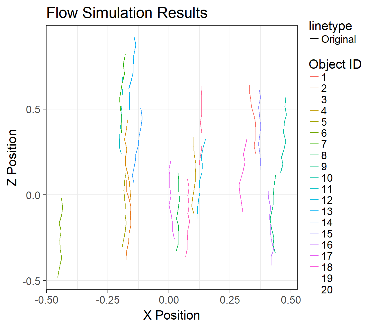
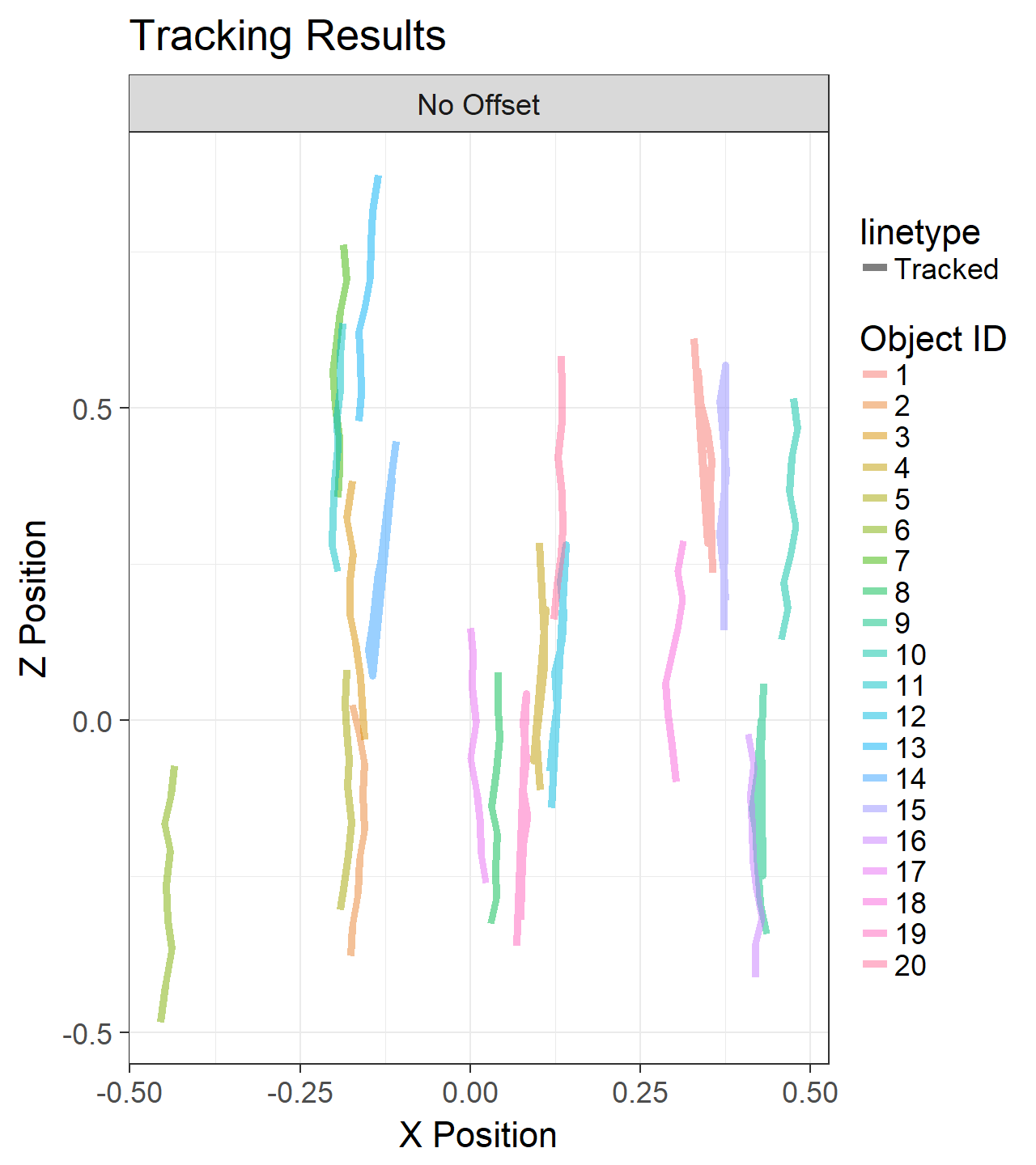
Limits of Tracking
We see that visually tracking samples can be difficult and there are a number of parameters which affect the ability for us to clearly see the tracking.
- flow rate
- flow type
- density
- appearance and disappearance rate
- jitter
- particle uniqueness
How to improve tracking
We have to try to quantify the limits of these parameters for different tracking methods in order to design experiments better.
Acquisition-based Parameters
- Acquisition rate
- flow rate vs. sampling rate
- jitter (per frame)
- Resolution
- density,
- appearance rate
Experimental Parameters
- Experimental setup (pressure, etc) $\rightarrow$ flow rate/type
- Polydispersity $\rightarrow$ particle uniqueness
- Vibration/temperature $\rightarrow$ jitter
- Mixture $\rightarrow$ density contrast
Basic Simulations
Input flow from simulation
$$ \vec{v}(\vec{x})=\langle 0,0,0.05 \rangle+||0.01||\measuredangle b $$
|
 |
Designing Experiments
How does this help us to design experiments?
- density can be changed by adjusting the concentration of the substances being examined or the field of view
- flow per frame (image velocity) can usually be adjusted by changing pressure or acquisition time
- jitter can be estimated from images
How much is enough?
Difficult to create one number for every experiment
5% error in bubble position $\rightarrow$
- <5% in flow field
- >20% error in topology
5% error in shape or volume $\rightarrow$
- 5% in distribution or changes
- > 5% in individual bubble changes
- > 15% for single bubble strain tensor calculations
Extending Nearest Neighbor
Bijective Requirement
We define $\vec{P}_f$ as the result of performing the nearest neigbhor tracking on $\vec{P}_0$ $$ \vec{P}_f=\textrm{argmin}(||\vec{P}_0-\vec{y} || \forall \vec{y}\in I_1) $$
We define $\vec{P}_i$ as the result of performing the nearest neigbhor tracking on $\vec{P}_f$ $$ \vec{P}_i=\textrm{argmin}(||\vec{P}_f-\vec{y} || \forall \vec{y}\in I_0) $$
We say the tracking is bijective if these two points are the same $$ \vec{P}_i \stackrel{?}{=} \vec{P}_0 $$
Maximum Displacement
$$ \vec{P}_1=\begin{cases} ||\vec{P}_0-\vec{y} ||<\textrm{MAXD}, & \textrm{argmin}(||\vec{P}_0-\vec{y} || \forall \vec{y}\in I_1) \\ \textrm{Otherwise}, & \emptyset \end{cases}$$Extending Nearest Neighbor (Continued)
Models of movement behavior to support tracking
Prior / Expected Movement
$$\vec{P}_1=\textrm{argmin}(||\vec{P}_0+\vec{v}_{offset}-\vec{y} || \forall \vec{y}\in I_1)$$Adaptive Movement
Can then be calculated in an iterative fashion where the offset is the average from all of the $\vec{P}_1-\vec{P}_0$ vectors. It can also be performed $$ \vec{P}_1=\textrm{argmin}(||\vec{P}_0+\vec{v}_{offset}-\vec{y} || \forall \vec{y}\in I_1) $$
More advanced models
- Use expected physical model
- Use track derivative to find $v_{offset}$
- Kalman filters can be used for particle tracking
Beyond Nearest Neighbor
While nearest neighbor
- provides a useful starting tool
- it is not sufficient for truly complicated flows and datasets.
Better Approaches
Multiple Hypothesis Testing
Nearest neighbor just compares the points between two frames and there is much more information available in most time-resolved datasets.
This approach allows for multiple possible paths to be explored at the same time and the best chosen only after all frames have been examined
Shortcomings
Merging and Splitting Particles
- The simplicity of the nearest neighbor model does really allow for particles to merge and split (relaxing the bijective requirement allows such behavior, but the method is still not suited for such tracking).
- For such systems a more specific, physically-based is required to encapsulate this behavior.
Voxel-based Approaches
Voxel-based Approaches
For voxel-based approachs the most common analyses are digital image correlation (or for 3D images digital volume correlation), where the correlation is calculated between two images or volumes.
Standard Image Correlation
Given images $I_0(\vec{x})$ and $I_1(\vec{x})$ at time $t_0$ and $t_1$ respectively. The correlation between these two images can be calculated for each $\vec{r}$
$$ C_{I_0,I_1}(\vec{r})=\langle I_0(\vec{x}) I_1(\vec{x}+\vec{r}) \rangle $$This can also be done in the Fourier space
$$C_{I_0,I_1}(\vec{r})=\mathcal{F}^{-1}\{\mathcal{F}\{I_0\}\cdot \mathcal{F}\{I_1\}^{*}\}$$Let's make some test data
We use a 'five' from the MNIST data set of handwritten numbers
import numpy as np
import matplotlib.pyplot as plt
from skimage.io import imread
%matplotlib inline
bw_img = np.load('../common/data/five.npy') # A 'five' from the mnist data set
shift_img = np.roll(np.roll(bw_img, -3, axis=0), 2, axis=1)
fig, (ax1, ax2) = plt.subplots(1, 2, figsize=(12, 6), dpi=100)
sns.heatmap(bw_img, ax=ax1, cbar=False, annot=True, fmt='d', cmap='bone'), ax1.set_title('$T_0$')
sns.heatmap(shift_img, ax=ax2, cbar=False, annot=True, fmt='d', cmap='bone') , ax2.set_title('$T_1$ ($T_0$ shifted by (-3,2))');

Demonstration of the correlation in space
from matplotlib.animation import FuncAnimation
from IPython.display import HTML
fig, (ax1, ax2, ax3) = plt.subplots(1, 3, figsize=(15, 5))
mx, my = np.meshgrid(np.arange(-4, 6, 2),
np.arange(-4, 6, 2))
nx = mx.ravel()
ny = my.ravel()
out_score = np.zeros(nx.shape, dtype=np.float32)
def update_frame(i):
a_img = bw_img
b_img = np.roll(np.roll(shift_img, nx[i], axis=1), ny[i], axis=0)
ax1.cla()
sns.heatmap(a_img, ax=ax1, cbar=False, annot=True, fmt='d', cmap='bone')
ax2.cla()
sns.heatmap(b_img, ax=ax2, cbar=False, annot=True, fmt='d', cmap='bone')
out_score[i] = np.mean(a_img*b_img)
ax3.cla()
sns.heatmap(out_score.reshape(mx.shape), ax=ax3,
cbar=False, annot=True, fmt='2.1f', cmap='RdBu')
ax3.set_xticklabels(mx[0, :])
ax3.set_yticklabels(my[:, 0])
ax1.set_title('Iteration #{}'.format(i+1))
ax2.set_title('X-Offset: %d\nY-Offset: %d' % (nx[i], ny[i]))
ax3.set_title(r'$\langle I_0(\vec{x}) I_1(\vec{x}+\vec{r}) \rangle$')
# write animation frames
anim_code = FuncAnimation(fig,
update_frame,
frames=len(nx),
interval=300,
repeat_delay=4000).to_html5_video()
plt.close('all')
HTML(anim_code)
fig, (ax1, ax2, ax3) = plt.subplots(1, 3, figsize=(15, 6))
out_score = np.zeros(nx.shape, dtype=np.float32)
for i in range(len(nx)):
a_img = bw_img
b_img = np.roll(np.roll(shift_img, nx[i], axis=1), ny[i], axis=0)
out_score[i] = np.mean(np.square(a_img-b_img))
# get the minimum
i_min = np.argmin(out_score)
b_img = np.roll(np.roll(shift_img, nx[i_min], axis=1), ny[i_min], axis=0)
sns.heatmap(a_img, ax=ax1, cbar=False, annot=True, fmt='d', cmap='bone')
sns.heatmap(b_img, ax=ax2, cbar=False, annot=True, fmt='d', cmap='bone')
sns.heatmap(out_score.reshape(mx.shape), ax=ax3, cbar=False,
annot=True, fmt='2.1f', cmap='viridis')
ax3.set_xticklabels(mx[0, :])
ax3.set_yticklabels(my[:, 0])
ax1.set_title('Iteration #{}'.format(i+1))
ax2.set_title('X-Offset: %d\nY-Offset: %d' % (nx[i_min], ny[i_min]))
ax3.set_title(r'$\langle (I_0(\vec{x})-I_1(\vec{x}+\vec{r}))^2 \rangle$');

Correlation using the Fourier transform
$$C_{I_0,I_1}(\vec{r})=\mathcal{F}^{-1}\{\mathcal{F}\{I_0\}\cdot \mathcal{F}\{I_1\}^{*}\}$$plt.figure(figsize=(15,8))
plt.subplot(2,3,1); plt.imshow(bw_img); plt.title('Image A')
plt.subplot(2,3,4); plt.imshow(shift_img); plt.title('Image B')
fa=(np.fft.fft2(bw_img));
fb=(np.fft.fft2(shift_img));
plt.subplot(2,3,2); plt.imshow(np.abs(np.fft.fftshift(fa))); plt.title('$|\mathcal{F}(A)|$')
plt.subplot(2,3,5); plt.imshow(np.abs(np.fft.fftshift(fb))); plt.title('$|\mathcal{F}(B)|$')
f=fa*np.conjugate(fb);
co=np.abs(np.fft.fftshift(np.fft.ifft2(f)));
plt.subplot(1,3,3)
plt.imshow(np.abs(co), extent = [-7 , 6, 6 , -7], cmap='viridis');plt.title('Correlation image between a and b');

import numpy as np
from skimage.filters import median
import seaborn as sns
import matplotlib.pyplot as plt
from skimage.io import imread
%matplotlib inline
full_img = imread("ext-figures/bonegfiltslice.png")
full_shift_img = median(
np.roll(np.roll(full_img, -15, axis=0), 15, axis=1), np.ones((1, 3)))
def g_roi(x): return x[5:90, 150:275]
bw_img = g_roi(full_img)
shift_img = g_roi(full_shift_img)
fig, (ax1, ax2) = plt.subplots(1, 2, figsize=(20, 6), dpi=100)
ax1.imshow(bw_img, cmap='bone'),ax1.set_title('Image $T_0$')
ax2.imshow(shift_img, cmap='bone'),ax2.set_title('Image $T_1$');

Let's look at a smaller region
fig, (ax1, ax2) = plt.subplots(1, 2, figsize=(20, 6), dpi=100)
def g_roi(x): return x[20:30, 210:225]
sns.heatmap(g_roi(full_img), ax=ax1, cbar=False,
annot=True, fmt='d', cmap='bone'), ax1.set_title('Image $T_0$')
sns.heatmap(g_roi(full_shift_img), ax=ax2, cbar=False,
annot=True, fmt='d', cmap='bone'); ax2.set_title('Image $T_1$');

from matplotlib.animation import FuncAnimation
from IPython.display import HTML
fig, (ax1, ax2, ax3) = plt.subplots(1, 3, figsize=(12, 4))
def g_roi(x): return x[20:30:2, 210:225:2]
mx, my = np.meshgrid(np.arange(-10, 12, 4),
np.arange(-10, 12, 4))
nx = mx.ravel()
ny = my.ravel()
out_score = np.zeros(nx.shape, dtype=np.float32)
def update_frame(i):
a_img = g_roi(full_img)
b_img = g_roi(np.roll(np.roll(full_shift_img, nx[i], axis=1), ny[i], axis=0))
ax1.cla(), sns.heatmap(a_img, ax=ax1, cbar=False, annot=True, fmt='d', cmap='bone')
ax2.cla(), sns.heatmap(b_img, ax=ax2, cbar=False, annot=True, fmt='d', cmap='bone')
out_score[i] = np.mean(np.square(a_img-b_img))
ax3.cla(), sns.heatmap(out_score.reshape(mx.shape), ax=ax3, cbar=False, annot=True, fmt='2.1f', cmap='RdBu')
ax1.set_title('Iteration #{}'.format(i+1))
ax2.set_title('X-Offset: %d\nY-Offset: %d' % (2*nx[i], 2*ny[i]))
ax3.set_xticklabels(mx[0, :])
ax3.set_yticklabels(my[:, 0])
# write animation frames
anim_code = FuncAnimation(fig,
update_frame,
frames=len(nx),
interval=300,
repeat_delay=2000).to_html5_video()
plt.close('all')
HTML(anim_code)
fig, (ax1, ax2, ax3) = plt.subplots(1, 3, figsize=(14, 6), dpi=100)
mx, my = np.meshgrid(np.arange(-20, 25, 5),
np.arange(-20, 25, 5))
nx = mx.ravel()
ny = my.ravel()
out_score = np.zeros(nx.shape, dtype=np.float32)
out_score = np.zeros(nx.shape, dtype=np.float32)
def g_roi(x): return x[5:90, 150:275]
for i in range(len(nx)):
a_img = g_roi(full_img)
b_img = g_roi(
np.roll(np.roll(full_shift_img, nx[i], axis=1), ny[i], axis=0))
out_score[i] = np.mean(np.square(a_img-b_img))
# get the minimum
i_min = np.argmin(out_score)
b_img = g_roi(np.roll(np.roll(full_shift_img, nx[i_min], axis=1), ny[i_min], axis=0))
ax1.imshow(a_img, cmap='bone'), ax1.set_title('$T_0$')
ax2.imshow(b_img, cmap='bone'), ax2.set_title('$T_1$ Registered')
sns.heatmap(out_score.reshape(mx.shape), ax=ax3, cbar=False,annot=True, fmt='2.1f', cmap='viridis')
ax3.set_xticklabels(mx[0, :]), ax3.set_yticklabels(my[:, 0])
ax1.set_title('Iteration #{}'.format(i+1))
ax2.set_title('X-Offset: %d\nY-Offset: %d' % (nx[i_min], ny[i_min]))
ax3.set_title(r'$\langle (I_0(\vec{x})-I_1(\vec{x}+\vec{r}))^2 \rangle$');

Registration
Registration
Before any meaningful tracking tasks can be performed, the first step is to register the measurements so they are all on the same coordinate system.
Often the registration can be done along with the tracking by separating the movement into actual sample movement and other (camera, setup, etc) if the motion of either the sample or the other components can be well modeled.
In medicine this is frequently needed because different scanners produce different kinds of outputs with different scales, positioning and resolutions. This is also useful for 'follow-up' scans with patients to identify how a disease has progressed. With scans like chest X-rays it isn't uncommon to have multiple (some patients have hundreds) all taken under different conditions

The Process
We informally followed a process before when trying to match the two images together, but we want to make this more generic for a larger spectrum of problems.
We thus follow the model set forward by tools like ITK with the components divided into the input data:
- Moving Image
- and Fixed Image sometimes called Reference Image).
The algorithmic components
- The Transform operation to transform the moving image.
- The interpolator to handle bringing all of the points onto a pixel grid.
- The Metric which is the measure of how well the transformed moving image and fixed image match
- and finally the Optimizer that tries to find the best solution
from IPython.display import SVG
from subprocess import check_output
import pydot
import os
def show_graph(graph):
try:
return SVG(graph.create_svg())
except AttributeError as e:
output = check_output('dot -Tsvg', shell=True,
input=g.to_string().encode())
return SVG(output.decode())
g = pydot.Graph(graph_type='digraph')
fixed_img = pydot.Node('Fixed Image\nReference Image',
shape='folder', style="filled", fillcolor="lightgreen")
moving_img = pydot.Node('Moving Image', shape='folder',
style="filled", fillcolor="lightgreen")
trans_obj = pydot.Node('Transform', shape='box',
style='filled', fillcolor='yellow')
g.add_node(fixed_img)
g.add_node(moving_img)
g.add_node(trans_obj)
g.add_edge(pydot.Edge(fixed_img, 'Metric'))
g.add_edge(pydot.Edge(moving_img, 'Interpolator'))
g.add_edge(pydot.Edge(trans_obj, 'Interpolator', label='Transform Parameters'))
g.add_edge(pydot.Edge('Interpolator', 'Metric'))
show_graph(g)
g.add_edge(pydot.Edge('Metric', 'Optimizer'))
g.add_edge(pydot.Edge('Optimizer', trans_obj))
show_graph(g)
Transform
The transform specifies the transformations which can take place on the moving image, a number of different types are possible, but the most frequent types are listed below.
- Affine
- Translation
- Scaling
- Deformable
- Shearing
Interpolator
The interpolator is the component applies the transform to the moving image. The common ways of interpolating are
- Nearest Neighbor
- Bilinear
- Bicubic
- Bspline
- ...
Metric
The metric is how the success of the matching of the two images is measured. The goal is to measure similarity between images.
- Mean Squared Error - the simplist metric to use just recording the raw difference, but often this can lead to unusual matches since noise and uneven illumination can lead to high MSE for images that match well.
- SSIM similarity metric
- Correlation Factor
Optimizer
The optimizer component is responsible for updating the parameters based on the metric. A standard approach with this is gradient descent where the gradient is calculated and a small step (determined by the learning rate) is taken in the direction of maximum descent.
- Gradient Descent
- Adam
- Stochastic Gradient Descent
- AdaGrad
- AdaDelta
Our tracker
g = pydot.Graph(graph_type='digraph')
fixed_img = pydot.Node('Fixed Image\nReference Image',
shape='folder', style="filled", fillcolor="lightgreen")
moving_img = pydot.Node('Moving Image', shape='folder',
style="filled", fillcolor="lightgreen")
trans_obj = pydot.Node('Transform', shape='box',
style='filled', fillcolor='yellow')
g.add_node(fixed_img)
g.add_node(moving_img)
g.add_node(trans_obj)
g.add_edge(pydot.Edge(fixed_img, 'Metric\nMean Squared Error'))
g.add_edge(pydot.Edge(moving_img, 'Interpolator\nNearest Neighbor'))
g.add_edge(pydot.Edge(trans_obj, 'Interpolator\nNearest Neighbor',
label='Transform Parameters'))
g.add_edge(pydot.Edge('Interpolator\nNearest Neighbor',
'Metric\nMean Squared Error'))
#g.add_edge(pydot.Edge('Metric\nMean Squared Error', 'Optimizer\nGrid Search', style = ''))
g.add_edge(pydot.Edge('Optimizer\nGrid Search', trans_obj))
show_graph(g)
Registration of the bone image
import numpy as np
from skimage.filters import median
import seaborn as sns
import matplotlib.pyplot as plt
from skimage.io import imread
%matplotlib inline
full_img = imread("ext-figures/bonegfiltslice.png")
full_shift_img = median(
np.roll(np.roll(full_img, -15, axis=0), 15, axis=1), np.ones((1, 3)))
def g_roi(x): return x[5:90, 150:275]
bw_img = g_roi(full_img)
shift_img = g_roi(full_shift_img)
fig, (ax1, ax2) = plt.subplots(1, 2, figsize=(20, 6), dpi=100)
ax1.imshow(bw_img, cmap='bone')
ax1.set_title('$T_0$')
ax2.imshow(shift_img, cmap='bone')
ax2.set_title('$T_1$');

#import tensorflow as tf
import tensorflow.compat.v1 as tf
tf.disable_v2_behavior()
from affine_op import affine_transform
g = tf.Graph()
with g.as_default():
init = tf.global_variables_initializer()
# tf Graph Input
fixed_img = tf.placeholder("float", shape=(
1, None, None, 1), name='FixedImage')
moving_img = tf.placeholder("float", shape=(
1, None, None, 1), name='MovingImage')
# Initialize the variables (i.e. assign their default value)
with tf.name_scope('transform_parameters'): # Set transform parameters
x_offset = tf.Variable(0.0, name="x_offset")
y_offset = tf.Variable(0.0, name="y_offset")
# we keep scale and rotation fixed
scale = tf.placeholder("float", shape=tuple(), name="scale")
rotation = tf.placeholder("float", shape=tuple(), name="rotation")
with tf.name_scope('transformer_and_interpolator'):
flat_mat = tf.tile([tf.cos(rotation), -tf.sin(rotation), x_offset,
tf.sin(rotation), tf.cos(rotation), y_offset], (1,))
flat_mat = tf.reshape(flat_mat, (1, 6))
trans_tensor = affine_transform(moving_img, flat_mat)
with tf.name_scope('metric'):
mse = tf.reduce_mean(
tf.square(fixed_img-trans_tensor), name='MeanSquareError')
optimizer = tf.train.GradientDescentOptimizer(1e-5).minimize(mse)
C:\Users\ander\anaconda3\lib\site-packages\tensorflow\python\framework\dtypes.py:516: FutureWarning: Passing (type, 1) or '1type' as a synonym of type is deprecated; in a future version of numpy, it will be understood as (type, (1,)) / '(1,)type'.
_np_qint8 = np.dtype([("qint8", np.int8, 1)])
C:\Users\ander\anaconda3\lib\site-packages\tensorflow\python\framework\dtypes.py:517: FutureWarning: Passing (type, 1) or '1type' as a synonym of type is deprecated; in a future version of numpy, it will be understood as (type, (1,)) / '(1,)type'.
_np_quint8 = np.dtype([("quint8", np.uint8, 1)])
C:\Users\ander\anaconda3\lib\site-packages\tensorflow\python\framework\dtypes.py:518: FutureWarning: Passing (type, 1) or '1type' as a synonym of type is deprecated; in a future version of numpy, it will be understood as (type, (1,)) / '(1,)type'.
_np_qint16 = np.dtype([("qint16", np.int16, 1)])
C:\Users\ander\anaconda3\lib\site-packages\tensorflow\python\framework\dtypes.py:519: FutureWarning: Passing (type, 1) or '1type' as a synonym of type is deprecated; in a future version of numpy, it will be understood as (type, (1,)) / '(1,)type'.
_np_quint16 = np.dtype([("quint16", np.uint16, 1)])
C:\Users\ander\anaconda3\lib\site-packages\tensorflow\python\framework\dtypes.py:520: FutureWarning: Passing (type, 1) or '1type' as a synonym of type is deprecated; in a future version of numpy, it will be understood as (type, (1,)) / '(1,)type'.
_np_qint32 = np.dtype([("qint32", np.int32, 1)])
C:\Users\ander\anaconda3\lib\site-packages\tensorflow\python\framework\dtypes.py:525: FutureWarning: Passing (type, 1) or '1type' as a synonym of type is deprecated; in a future version of numpy, it will be understood as (type, (1,)) / '(1,)type'.
np_resource = np.dtype([("resource", np.ubyte, 1)])
WARNING:tensorflow:From C:\Users\ander\anaconda3\lib\site-packages\tensorflow\python\compat\v2_compat.py:61: disable_resource_variables (from tensorflow.python.ops.variable_scope) is deprecated and will be removed in a future version. Instructions for updating: non-resource variables are not supported in the long term
C:\Users\ander\anaconda3\lib\site-packages\tensorboard\compat\tensorflow_stub\dtypes.py:541: FutureWarning: Passing (type, 1) or '1type' as a synonym of type is deprecated; in a future version of numpy, it will be understood as (type, (1,)) / '(1,)type'.
_np_qint8 = np.dtype([("qint8", np.int8, 1)])
C:\Users\ander\anaconda3\lib\site-packages\tensorboard\compat\tensorflow_stub\dtypes.py:542: FutureWarning: Passing (type, 1) or '1type' as a synonym of type is deprecated; in a future version of numpy, it will be understood as (type, (1,)) / '(1,)type'.
_np_quint8 = np.dtype([("quint8", np.uint8, 1)])
C:\Users\ander\anaconda3\lib\site-packages\tensorboard\compat\tensorflow_stub\dtypes.py:543: FutureWarning: Passing (type, 1) or '1type' as a synonym of type is deprecated; in a future version of numpy, it will be understood as (type, (1,)) / '(1,)type'.
_np_qint16 = np.dtype([("qint16", np.int16, 1)])
C:\Users\ander\anaconda3\lib\site-packages\tensorboard\compat\tensorflow_stub\dtypes.py:544: FutureWarning: Passing (type, 1) or '1type' as a synonym of type is deprecated; in a future version of numpy, it will be understood as (type, (1,)) / '(1,)type'.
_np_quint16 = np.dtype([("quint16", np.uint16, 1)])
C:\Users\ander\anaconda3\lib\site-packages\tensorboard\compat\tensorflow_stub\dtypes.py:545: FutureWarning: Passing (type, 1) or '1type' as a synonym of type is deprecated; in a future version of numpy, it will be understood as (type, (1,)) / '(1,)type'.
_np_qint32 = np.dtype([("qint32", np.int32, 1)])
C:\Users\ander\anaconda3\lib\site-packages\tensorboard\compat\tensorflow_stub\dtypes.py:550: FutureWarning: Passing (type, 1) or '1type' as a synonym of type is deprecated; in a future version of numpy, it will be understood as (type, (1,)) / '(1,)type'.
np_resource = np.dtype([("resource", np.ubyte, 1)])
import numpy as np
from IPython.display import clear_output, Image, display, HTML
def strip_consts(graph_def, max_const_size=32):
"""Strip large constant values from graph_def."""
strip_def = tf.GraphDef()
for n0 in graph_def.node:
n = strip_def.node.add()
n.MergeFrom(n0)
if n.op == 'Const':
tensor = n.attr['value'].tensor
size = len(tensor.tensor_content)
if size > max_const_size:
tensor.tensor_content = "<stripped %d bytes>" % size
return strip_def
def show_graph(graph_def, max_const_size=32):
"""Visualize TensorFlow graph."""
if hasattr(graph_def, 'as_graph_def'):
graph_def = graph_def.as_graph_def()
strip_def = strip_consts(graph_def, max_const_size=max_const_size)
code = """
<script src="//cdnjs.cloudflare.com/ajax/libs/polymer/0.3.3/platform.js"></script>
<script>
function load() {{
document.getElementById("{id}").pbtxt = {data};
}}
</script>
<link rel="import" href="https://tensorboard.appspot.com/tf-graph-basic.build.html" onload=load()>
<div style="height:600px">
<tf-graph-basic id="{id}"></tf-graph-basic>
</div>
""".format(data=repr(str(strip_def)), id='graph'+str(np.random.rand()))
iframe = """
<iframe seamless style="width:1200px;height:620px;border:0" srcdoc="{}"></iframe>
""".format(code.replace('"', '"'))
display(HTML(iframe))
show_graph(g)
# Start training
from matplotlib.animation import FuncAnimation
from IPython.display import HTML
import numpy as np
def make_feed_dict(f_img, m_img):
return {fixed_img: np.expand_dims(np.expand_dims(f_img, 0), -1),
moving_img: np.expand_dims(np.expand_dims(m_img, 0), -1),
rotation: 0.0}
loss_history = []
optimize_iters = 10
with tf.Session(graph=g) as sess:
plt.close('all')
fig, m_axs = plt.subplots(2, 2, figsize=(10, 10), dpi=100)
#tf.initialize_all_variables().run()
init = tf.global_variables_initializer()
# Run the initializer
sess.run(init)
# Fit all training data
const_feed_dict = make_feed_dict(bw_img, shift_img)
def update_frame(i):
global loss_history
(ax1, ax2), (ax4, ax3) = m_axs
for c_ax in m_axs.flatten():
c_ax.cla()
c_ax.axis('off')
f_mse, x_pos, y_pos, rs_img = sess.run([mse, x_offset, y_offset, trans_tensor],
feed_dict=const_feed_dict)
loss_history += [f_mse]
ax1.imshow(bw_img, cmap='bone')
ax1.set_title('$T_0$')
ax2.imshow(shift_img, cmap='bone')
ax2.set_title('$T_1$')
#ax3.imshow(rs_img[0,:,:,0], cmap = 'bone')
# ax3.set_title('Output')
ax4.imshow(bw_img*1.0-rs_img[0, :, :, 0],
cmap='RdBu', vmin=-100, vmax=100)
ax4.set_title('Difference\nMSE: %2.2f' % (f_mse))
ax3.semilogy(loss_history)
ax3.set_xlabel('Iteration')
ax3.set_ylabel('MSE (Log-scale)')
ax3.axis('on')
for _ in range(1):
sess.run(optimizer, feed_dict=const_feed_dict)
# write animation frames
anim_code = FuncAnimation(fig,
update_frame,
frames=optimize_iters,
interval=1000,
repeat_delay=2000).to_html5_video()
plt.close('all')
HTML(anim_code)
g_roi = tf.Graph()
with g_roi.as_default():
init = tf.global_variables_initializer()
# tf Graph Input
fixed_img = tf.placeholder("float", shape=(
1, None, None, 1), name='FixedImage')
moving_img = tf.placeholder("float", shape=(
1, None, None, 1), name='MovingImage')
# Initialize the variables (i.e. assign their default value)
with tf.name_scope('transform_parameters'): # Set transform parameters
x_offset = tf.Variable(0.0, name="x_offset")
y_offset = tf.Variable(0.0, name="y_offset")
# we keep rotation fixed
rotation = tf.placeholder("float", shape=tuple(), name="rotation")
with tf.name_scope('transformer_and_interpolator'):
flat_mat = tf.tile([tf.cos(rotation), -tf.sin(rotation), x_offset,
tf.sin(rotation), tf.cos(rotation), y_offset], (1,))
flat_mat = tf.reshape(flat_mat, (1, 6))
trans_tensor = affine_transform(moving_img, flat_mat)
with tf.name_scope('metric'):
diff_tensor = (fixed_img-trans_tensor)[:, 25:75, 25:110, :]
mse = tf.reduce_mean(tf.square(diff_tensor), name='MeanSquareError')
optimizer = tf.train.GradientDescentOptimizer(2e-6).minimize(mse)
# Start training
from matplotlib.animation import FuncAnimation
from IPython.display import HTML
from matplotlib import patches
optimize_iters = 20
loss_history = []
with tf.Session(graph=g_roi) as sess:
plt.close('all')
fig, m_axs = plt.subplots(2, 3, figsize=(9, 4), dpi=100)
init = tf.global_variables_initializer()
# Run the initializer
sess.run(init)
# Fit all training data
const_feed_dict = make_feed_dict(bw_img, shift_img)
def update_frame(i):
global loss_history
(ax1, ax2, ax5), (ax3, ax4, ax6) = m_axs
for c_ax in m_axs.flatten():
c_ax.cla()
c_ax.axis('off')
f_mse, x_pos, y_pos, rs_img, diff_img = sess.run([mse, x_offset, y_offset, trans_tensor, diff_tensor],
feed_dict=const_feed_dict)
loss_history += [f_mse]
ax1.imshow(bw_img, cmap='bone')
ax1.set_title('$T_0$')
ax2.imshow(shift_img, cmap='bone')
ax2.set_title('$T_1$')
ax3.imshow(rs_img[0, :, :, 0], cmap='bone')
ax3.set_title('Output')
ax4.imshow(bw_img*1.0-rs_img[0, :, :, 0],
cmap='RdBu', vmin=-100, vmax=100)
ax4.set_title('MSE: %2.2f' % (f_mse))
rect = patches.Rectangle(
(25, 25), 85, 50, linewidth=2, edgecolor='g', facecolor='none')
# Add the patch to the Axes
ax4.add_patch(rect)
ax5.semilogy(loss_history)
ax5.set_xlabel('Iteration')
ax5.set_ylabel('MSE (Log-scale)')
ax5.axis('on')
ax6.imshow(diff_img[0, :, :, 0], cmap='RdBu', vmin=-100, vmax=100)
ax6.set_title('ROI')
for _ in range(5):
sess.run(optimizer, feed_dict=const_feed_dict)
# write animation frames
anim_code = FuncAnimation(fig,
update_frame,
frames=optimize_iters,
interval=1000,
repeat_delay=2000).to_html5_video()
plt.close('all')
HTML(anim_code)
Smoother Gradient
We can use a distance map of the segmentation to give us a smoother gradient
from scipy.ndimage import distance_transform_edt
from skimage.filters import threshold_otsu
fig, [(ax1, ax2), (ax3, ax4)] = plt.subplots(2, 2, figsize=(8, 8))
thresh_img = bw_img > threshold_otsu(bw_img)
dist_start_img = distance_transform_edt(thresh_img)
dist_shift_img = distance_transform_edt(shift_img > threshold_otsu(bw_img))
ax1.imshow(bw_img, cmap='bone')
ax2.imshow(thresh_img, cmap='bone')
ax3.imshow(dist_start_img, cmap='jet')
ax3.set_title('dmap Fixed Image')
ax4.imshow(dist_shift_img, cmap='jet')
ax4.set_title('dmap Moving Image');

# Start training
from matplotlib.animation import FuncAnimation
from IPython.display import HTML
from matplotlib import patches
optimize_iters = 20
loss_history = []
with tf.Session(graph=g_roi) as sess:
plt.close('all')
fig, m_axs = plt.subplots(2, 3, figsize=(12, 4), dpi=100)
# Run the initializer
tf.initialize_all_variables().run()
# Fit all training data
const_feed_dict = make_feed_dict(dist_start_img, dist_shift_img)
real_image_feed_dict = make_feed_dict(bw_img, shift_img)
def update_frame(i):
global loss_history
(ax1, ax2, ax5), (ax3, ax4, ax6) = m_axs
for c_ax in m_axs.flatten():
c_ax.cla()
c_ax.axis('off')
f_mse, x_pos, y_pos, rs_img, diff_img = sess.run([mse, x_offset, y_offset, trans_tensor, diff_tensor],
feed_dict=const_feed_dict)
real_rs_img, real_diff_img = sess.run([trans_tensor, diff_tensor],
feed_dict=real_image_feed_dict)
loss_history += [f_mse]
ax1.imshow(bw_img, cmap='bone')
ax1.set_title('$T_0$')
ax2.imshow(shift_img, cmap='bone')
ax2.set_title('$T_1$')
ax3.imshow(real_rs_img[0, :, :, 0], cmap='bone')
ax3.set_title('Output')
ax4.imshow(dist_start_img*1.0 -
rs_img[0, :, :, 0], cmap='RdBu', vmin=-10, vmax=10)
ax4.set_title('MSE: %2.2f' % (f_mse))
rect = patches.Rectangle(
(25, 25), 75, 50, linewidth=2, edgecolor='g', facecolor='none')
# Add the patch to the Axes
ax4.add_patch(rect)
ax5.semilogy(loss_history)
ax5.set_xlabel('Iteration')
ax5.set_ylabel('MSE\n(Log-scale)')
ax5.axis('on')
ax6.imshow(diff_img[0, :, :, 0], cmap='RdBu', vmin=-10, vmax=10)
ax6.set_title('ROI')
for _ in range(200):
sess.run(optimizer, feed_dict=const_feed_dict)
# write animation frames
anim_code = FuncAnimation(fig,
update_frame,
frames=optimize_iters,
interval=1000,
repeat_delay=2000).to_html5_video()
plt.close('all')
HTML(anim_code)
WARNING:tensorflow:From C:\Users\ander\anaconda3\lib\site-packages\tensorflow\python\util\tf_should_use.py:193: initialize_all_variables (from tensorflow.python.ops.variables) is deprecated and will be removed after 2017-03-02. Instructions for updating: Use `tf.global_variables_initializer` instead.
Try structural similarity index metric
from backport_ssim import _ssim_per_channel
g_roi_ssim = tf.Graph()
with g_roi_ssim.as_default():
init = tf.global_variables_initializer()
# tf Graph Input
fixed_img = tf.placeholder("float", shape=(
1, None, None, 1), name='FixedImage')
moving_img = tf.placeholder("float", shape=(
1, None, None, 1), name='MovingImage')
# Initialize the variables (i.e. assign their default value)
with tf.name_scope('transform_parameters'): # Set transform parameters
x_offset = tf.Variable(0.0, name="x_offset")
y_offset = tf.Variable(0.0, name="y_offset")
# we keep rotation fixed
rotation = tf.placeholder("float", shape=tuple(), name="rotation")
with tf.name_scope('transformer_and_interpolator'):
flat_mat = tf.tile([tf.cos(rotation), -tf.sin(rotation), x_offset,
tf.sin(rotation), tf.cos(rotation), y_offset], (1,))
flat_mat = tf.reshape(flat_mat, (1, 6))
trans_tensor = affine_transform(moving_img, flat_mat)
with tf.name_scope('metric'):
ssim, _ = _ssim_per_channel(fixed_img[:, 20:75, 25:100, :]/255.0,
trans_tensor[:, 20:75, 25:100, :]/255.0,
max_val=1.0)
mssim = tf.reduce_mean(ssim, name='MeanSSIM')
rev_mssim = 1-mssim # since we can only minimize
optimizer = tf.train.GradientDescentOptimizer(5e-2).minimize(rev_mssim)
# Start training
from matplotlib.animation import FuncAnimation
from IPython.display import HTML
from matplotlib import patches
optimize_iters = 40
loss_history = []
with tf.Session(graph=g_roi_ssim) as sess:
plt.close('all')
fig, m_axs = plt.subplots(2, 3, figsize=(11, 5), dpi=100)
tf.initialize_all_variables().run()
# Run the initializer
sess.run(init)
# Fit all training data
const_feed_dict = make_feed_dict(bw_img, shift_img)
def update_frame(i):
global loss_history
(ax1, ax2, ax5), (ax3, ax4, ax6) = m_axs
for c_ax in m_axs.flatten():
c_ax.cla()
c_ax.axis('off')
f_ssim, x_pos, y_pos, rs_img = sess.run([mssim, x_offset, y_offset, trans_tensor],
feed_dict=const_feed_dict)
loss_history += [f_ssim]
ax1.imshow(bw_img, cmap='bone')
ax1.set_title('$T_0$')
ax2.imshow(shift_img, cmap='bone')
ax2.set_title('$T_1$')
ax3.imshow(rs_img[0, :, :, 0], cmap='bone')
ax3.set_title('Output')
ax4.imshow(bw_img*1.0-rs_img[0, :, :, 0],
cmap='RdBu', vmin=-100, vmax=100)
ax4.set_title('Difference\nSSIM: %2.2f' % (f_ssim))
rect = patches.Rectangle(
(25, 20), 75, 55, linewidth=2, edgecolor='g', facecolor='none')
# Add the patch to the Axes
ax4.add_patch(rect)
ax5.plot(loss_history)
ax5.set_xlabel('Iteration')
ax5.set_ylabel('SSIM')
ax5.axis('on')
for _ in range(1):
sess.run(optimizer, feed_dict=const_feed_dict)
# write animation frames
anim_code = FuncAnimation(fig,
update_frame,
frames=optimize_iters,
interval=1000,
repeat_delay=2000).to_html5_video()
plt.close('all')
HTML(anim_code)
ITK and Simple ITK
For medical imaging the standard tools used are ITK and SimpleITK and they have been optimized over decades to deliver high-performance registration tasks. They are a bit clumsy to use from python, but they offer by far the best established tools for these problems.
[https://itk.org/ITKSoftwareGuide/html/Book2/ITKSoftwareGuide-Book2ch3.html]
import SimpleITK as sitk
def register_img(fixed_arr,
moving_arr,
use_affine=True,
use_mse=True,
brute_force=True):
fixed_image = sitk.GetImageFromArray(fixed_arr)
moving_image = sitk.GetImageFromArray(moving_arr)
transform = sitk.AffineTransform(
2) if use_affine else sitk.ScaleTransform(2)
initial_transform = sitk.CenteredTransformInitializer(sitk.Cast(fixed_image, moving_image.GetPixelID()),
moving_image,
transform,
sitk.CenteredTransformInitializerFilter.GEOMETRY)
ff_img = sitk.Cast(fixed_image, sitk.sitkFloat32)
mv_img = sitk.Cast(moving_image, sitk.sitkFloat32)
registration_method = sitk.ImageRegistrationMethod()
if use_mse:
registration_method.SetMetricAsMeanSquares()
else:
registration_method.SetMetricAsMattesMutualInformation(
numberOfHistogramBins=50)
if brute_force:
sample_per_axis = 12
registration_method.SetOptimizerAsExhaustive(
[sample_per_axis//2, 0, 0])
# Utilize the scale to set the step size for each dimension
registration_method.SetOptimizerScales(
[2.0*3.14/sample_per_axis, 1.0, 1.0])
else:
registration_method.SetMetricSamplingStrategy(
registration_method.RANDOM)
registration_method.SetMetricSamplingPercentage(0.25)
registration_method.SetInterpolator(sitk.sitkLinear)
registration_method.SetOptimizerAsGradientDescent(learningRate=1.0,
numberOfIterations=200,
convergenceMinimumValue=1e-6,
convergenceWindowSize=10)
# Scale the step size differently for each parameter, this is critical!!!
registration_method.SetOptimizerScalesFromPhysicalShift()
registration_method.SetInitialTransform(initial_transform, inPlace=False)
final_transform_v1 = registration_method.Execute(ff_img,
mv_img)
print('Optimizer\'s stopping condition, {0}'.format(
registration_method.GetOptimizerStopConditionDescription()))
print('Final metric value: {0}'.format(
registration_method.GetMetricValue()))
resample = sitk.ResampleImageFilter()
resample.SetReferenceImage(fixed_image)
# SimpleITK supports several interpolation options, we go with the simplest that gives reasonable results.
resample.SetInterpolator(sitk.sitkBSpline)
resample.SetTransform(final_transform_v1)
return sitk.GetArrayFromImage(resample.Execute(moving_image))
%matplotlib inline
reg_img = register_img(bw_img, shift_img, brute_force=False, use_mse=True)
print(reg_img.max(), bw_img.max())
fig, (ax1, ax2, ax2d, ax3, ax4) = plt.subplots(1, 5, figsize=(20, 5), dpi=100)
ax1.imshow(bw_img, cmap='bone')
ax1.set_title('$T_0$')
ax2.imshow(shift_img, cmap='bone')
ax2.set_title('$T_1$')
ax2d.imshow(1.0*bw_img-shift_img, cmap='RdBu', vmin=-100, vmax=100)
ax2d.set_title('$T_1$ Registerd Difference')
ax3.imshow(reg_img, cmap='bone')
ax3.set_title('$T_1$ Registered')
ax4.imshow(1.0*bw_img-reg_img, cmap='RdBu', vmin=-127, vmax=127)
ax3.set_title('$T_1$ Registerd Difference');
Optimizer's stopping condition, GradientDescentOptimizerv4Template: Convergence checker passed at iteration 22. Final metric value: 1603.18885123802 255 255

Subdividing the data
We can approach the problem by subdividing the data into smaller blocks and then apply the digital volume correlation independently to each block.
- information on changes in different regions
- less statistics than a larger box
Introducing Physics
DIC or DVC by themselves include no sanity check for realistic offsets in the correlation itself. The method can, however be integrated with physical models to find a more optimal solutions.
- information from surrounding points
- smoothness criteria
- maximum deformation / force
- material properties
Distribution Metrics
As we covered before distribution metrics like the distribution tensor can be used for tracking changes inside a sample. Of these the most relevant is the texture tensor from cellular materials and liquid foam. The texture tensor is the same as the distribution tensor except that the edges (or faces) represent physically connected / touching objects rather than touching Voronoi faces (or conversely Delaunay triangles).
These metrics can also be used for tracking the behavior of a system without tracking the single points since most deformations of a system also deform the distribution tensor and can thus be extracted by comparing the distribution tensor at different time steps.
Quantifying Deformation: Strain
We can take any of these approaches and quantify the deformation using a tool called the strain tensor.
Strain is defined in mechanics for the simple 1D case as the change in the length against the change in the original length.
$$ e = \frac{\Delta L}{L} $$While this defines the 1D case well, it is difficult to apply such metrics to voxel, shape, and tensor data.
Strain Tensor
There are a number of different ways to calculate strain and the strain tensor, but the most applicable for general image based applications is called the infinitesimal strain tensor, because the element matches well to square pixels and cubic voxels.

Types of Strain
We catagorize the types of strain into two main catagories:
$$ \underbrace{\mathbf{E}}_{\textrm{Total Strain}} = \underbrace{\varepsilon_M \mathbf{I_3}}_{\textrm{Volumetric}} + \underbrace{\mathbf{E}^\prime}_{\textrm{Deviatoric}} $$Volumetric / Dilational
The isotropic change in size or scale of the object.
Deviatoric
The change in the proportions of the object (similar to anisotropy) independent of the final scale
Two Point Correlation - Volcanic Rock
Data provided by Mattia Pistone and Julie Fife
The air phase changes from small very anisotropic bubbles to one large connected pore network.
- The same tools cannot be used to quantify those systems.
- Furthermore there are motion artifacts which are difficult to correct.
We can utilize the two point correlation function of the material to characterize the shape generically for each time step and then compare.
Summary
- Dynamic experiments
- Object tracking
- Registration