Geospatial Data Science Applications: GEOG 4/590

Jan 24, 2022

Lecture 4: Gridded data

Johnny Ryan: jryan4@uoregon.edu

Content of this lecture¶

Quick review of raster data

* Bit of history about handling raster data in Python

* Introduce `GDAL`, `rasterio`, and `xarray` libararies

* Learn how to read, inspect, manipulate, and write raster data using these libraries

* Background for this week's lab

Raster data¶

Raster data represent a matrix of cells (or pixels) organized into rows and columns (or a grid)

Examples: surface maps¶

Grid cells can represent data that changes continuously across a landscape (surface) such as elevation or air temperature.

https://desktop.arcgis.com/en/arcmap/10.3/manage-data/raster-and-images/what-is-raster-data.htm

Examples: satellite imagery¶

Grid cells can represent from a satellite imagaing platforms such as reflectance.

Examples: classification maps¶

Grid cells can also represent discrete data (e.g. vegetation type or land cover).

Libraries¶

There is one library for accessing raster data:

The Geographic Raster Abstraction Library or GDAL

GDAL is written in C++ and ships with a C API.
ArcGIS, QGIS, Google Earth etc. all use GDAL to read/write/analyze raster data under-the-hood

GDAL¶

Supports read/write access for over 160 raster formats (e.g. GeoTIFF, NetCDF4)
Includes methods for:
- Finding dataset information
- Reprojecting
- Resampling
- Format conversion
- Mosaicking

Rasterio¶

Developed in 2016 with the goal of expressing GDAL's data model in a more Pythonic way
High performance, lower cognitive load, more transparent code

NumPy¶

Once we have read raster data in Python, we can apply fast matrix operations using numpy

xarray¶

Introduces labels in the form of dimensions, coordinates and attributes on top of raw NumPy-like arrays

Let's get started...¶

In [1]:

# Import libraries
import numpy as np
import rasterio

import matplotlib.pyplot as plt
from mpl_toolkits.axes_grid1 import make_axes_locatable

Open a raster file¶

Rasterio's open() function takes a path string and returns a dataset object.

The path may point to a file of any supported raster format.

Rasterio will open it using the proper GDAL format driver.

In [2]:

# Open raster file as dataset object
src = rasterio.open('data/N46W122.tif')
src

Out[2]:

<open DatasetReader name='data/N46W122.tif' mode='r'>

Dataset attributes¶

The dataset object contains a number of attributes which can be explored.

In [3]:

print("Number of bands:", src.count)

Number of bands: 1

A dataset band is an array of values representing a single variable in 2D space.

All band arrays of a dataset have the same number of rows and columns.

In [4]:

print("Width:", src.width)
print("Height:", src.height)

Width: 3601
Height: 3601

Dataset georeferencing¶

Raster data is different from an ordinary image because the pixels can be mapped to regions on the Earth's surface.

Every pixels of a dataset is contained within a spatial bounding box.

In [5]:

src.bounds

Out[5]:

BoundingBox(left=-122.00013888888888, bottom=45.999861111111116, right=-120.9998611111111, top=47.00013888888889)

The value of bounds attribute is derived from a more fundamental attribute: the dataset's geospatial transform.

In [6]:

src.transform

Out[6]:

Affine(0.0002777777777777778, 0.0, -122.00013888888888,
       0.0, -0.0002777777777777778, 47.00013888888889)

But what do these values represent? These coordinate values are relative to the origin of the dataset’s coordinate reference system (CRS).

In [7]:

src.crs

Out[7]:

CRS.from_epsg(4326)

In [8]:

src.transform

Out[8]:

Affine(0.0002777777777777778, 0.0, -122.00013888888888,
       0.0, -0.0002777777777777778, 47.00013888888889)

The georeferencing of a raster dataset can be fully described by the crs and transform attributes.

Reading raster data¶

Data from a raster band can be accessed by the band's index number. Following the GDAL convention, bands are indexed from 1.

In [9]:

# Read data in dataset object
srtm = src.read(1)

The read() method returns a numpy N-D array.

In [10]:

srtm

Out[10]:

array([[ 487,  485,  484, ..., 1729, 1738, 1747],
       [ 490,  489,  488, ..., 1718, 1727, 1733],
       [ 492,  491,  490, ..., 1704, 1713, 1721],
       ...,
       [ 976,  979,  980, ..., 1111, 1113, 1116],
       [ 975,  979,  979, ..., 1111, 1113, 1116],
       [ 971,  972,  974, ..., 1112, 1114, 1116]], dtype=int16)

In [11]:

# Plot data
fig, ax = plt.subplots(figsize=(8,8))
im = ax.imshow(srtm)
ax.set_title("Mt Rainier and Mt Adams", fontsize=14)
cbar = fig.colorbar(im, orientation='vertical')
cbar.ax.set_ylabel('Elevation', rotation=270, fontsize=14)
cbar.ax.get_yaxis().labelpad = 20

Indexing¶

Many GIS tasks require us to read a raster value at a given locations.

Dataset objects have an index() method for deriving the array indices corresponding to points in georeferenced space.

Let's demonstrate with an example... what is the elevation of the summit of Mt Rainier? (-121.760424, 46.852947)

In [12]:

# Define latitude and longitude of summit
rainier_summit = [-121.760424, 46.852947]

# Find row/column in corresponding raster dataset
loc_idx = src.index(rainier_summit[0], rainier_summit[1])

print("Grid cell index:", loc_idx)

Grid cell index: (529, 862)

In [13]:

# Read value from dataset object
elevation = srtm[loc_idx]

print("The summit of Mt Rainier is at %.0f m" %elevation)

print('... which is equivalent to %.0f ft' %(elevation * 3.281))

The summit of Mt Rainier is at 4374 m
... which is equivalent to 14351 ft

In [14]:

# Visualize
fig, ax = plt.subplots(figsize=(8,8))
im = ax.imshow(srtm)

# Plot a point on grid
ax.scatter(loc_idx[1], loc_idx[0], s=50, color='red')

ax.set_title("Mt Rainier and Mt Adams", fontsize=14)
cbar = fig.colorbar(im, orientation='vertical')
cbar.ax.set_ylabel('Elevation', rotation=270, fontsize=14)
cbar.ax.get_yaxis().labelpad = 20

More indexing methods¶

How would we find the index of the lowest elevation in this raster?

In [15]:

# .argmin() returns the indices of the minimum values of an array
min_value = srtm.argmin()
print(min_value)

In [16]:

# Convert 1D index to 2D coordinates
low_idx = np.unravel_index(min_value, srtm.shape)
print(low_idx)

(1683, 97)

In [17]:

# Find elevation value
elevation = srtm[low_idx]

print("The lowest elevation is %.0f m" %elevation)

The lowest elevation is 262 m

In [18]:

# Visualize data
fig, ax = plt.subplots(figsize=(7,7))
im = ax.imshow(srtm)

# Plot a point on grid
ax.scatter(loc_idx[1], loc_idx[0], s=50, color='red')
ax.scatter(low_idx[1], low_idx[0], s=50, color='orange')

ax.set_title("Mt Rainier and Mt Adams", fontsize=14)
cbar = fig.colorbar(im, orientation='vertical')
cbar.ax.set_ylabel('Elevation', rotation=270, fontsize=14)
cbar.ax.get_yaxis().labelpad = 20

Reprojecting¶

Rasterio can reproject raster data... but it's a bit of a mess!

Better to use GDAL command line tools.

t_srs stands for target spatial reference.

In [19]:

!gdalwarp -t_srs EPSG:32610 data/N46W122.tif data/N46W122_utm.tif

Processing data/N46W122.tif [1/1] : 0Using internal nodata values (e.g. -32768) for image data/N46W122.tif.
...10...20...30...40...50...60...70...80...90...100 - done.

We can execute terminal commands in jupyter notebook cells using !

In [20]:

src = rasterio.open('data/N46W122_utm.tif')
src.crs

Out[20]:

CRS.from_epsg(32610)

In [21]:

# Read data in file
srtm = src.read(1)

fig, ax = plt.subplots(figsize=(7,7))
im = ax.imshow(srtm)

ax.set_title("Mt Rainier and Mt Adams", fontsize=14)
cbar = fig.colorbar(im, orientation='vertical')
cbar.ax.set_ylabel('Elevation', rotation=270, fontsize=14)
cbar.ax.get_yaxis().labelpad = 20

Our data no longer represents a rectangle/square after reprojecting so we introduced some NoData values

In [22]:

srtm

Out[22]:

array([[-32768, -32768, -32768, ..., -32768, -32768, -32768],
       [-32768, -32768, -32768, ..., -32768, -32768, -32768],
       [-32768, -32768, -32768, ..., -32768, -32768, -32768],
       ...,
       [-32768, -32768, -32768, ..., -32768, -32768, -32768],
       [-32768, -32768, -32768, ..., -32768, -32768, -32768],
       [-32768, -32768, -32768, ..., -32768, -32768, -32768]], dtype=int16)

In [23]:

# Make NoData mask
srtm_masked = np.ma.masked_array(srtm, mask=(srtm == -32768))

fig, ax = plt.subplots(figsize=(7,7))
im = ax.imshow(srtm_masked)

ax.set_title("Mt Rainier and Mt Adams", fontsize=14)
cbar = fig.colorbar(im, orientation='vertical')
cbar.ax.set_ylabel('Elevation', rotation=270, fontsize=14)
cbar.ax.get_yaxis().labelpad = 20

Resampling¶

Is also easier with GDAL command line tools

In [24]:

!gdalwarp -tr 1000 -1000 data/N46W122_utm.tif data/N46W122_utm_1000.tif

Creating output file that is 79P x 113L.
Processing data/N46W122_utm.tif [1/1] : 0Using internal nodata values (e.g. -32768) for image data/N46W122_utm.tif.
Copying nodata values from source data/N46W122_utm.tif to destination data/N46W122_utm_1000.tif.
...10...20...30...40...50...60...70...80...90...100 - done.

-tr stands for target resolution

In [25]:

# Open new raster dataset
src = rasterio.open('data/N46W122_utm_1000.tif')

# Read new raster dataset
srtm_1000 = src.read(1)

# Mask data
srtm_1000_masked = np.ma.masked_array(srtm_1000, mask=(srtm_1000 == -32768))

In [26]:

# Plot 
fig, ax = plt.subplots(figsize=(8,8))
im = ax.imshow(srtm_1000_masked)

ax.set_title("Mt Rainier and Mt Adams", fontsize=14)
cbar = fig.colorbar(im, orientation='vertical')
cbar.ax.set_ylabel('Elevation', rotation=270, fontsize=14)
cbar.ax.get_yaxis().labelpad = 20

Multidimensional datasets¶

Sometimes we have raster data with a third or fourth dimension.

3D could represent multiple spectral bands or pressure levels, 4D often represents time

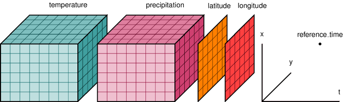
xarray is the recommended package for reading, writing, and analyzing scientific datasets stored in .nc or hdf format.

Scientific datasets include climate and satellite data.

In [27]:

# Import library
import xarray as xr

In [28]:

# Read data
xds = xr.open_dataset('data/era_jul_dec_2020.nc')

In [29]:

# Plot
fig, (ax1, ax2) = plt.subplots(ncols=2, figsize=(14,4))

im1 = ax1.imshow(xds['t2m'][0,:,:], cmap='RdYlBu_r')
im2 = ax2.imshow(xds['t2m'][1,:,:], cmap='RdYlBu_r')

ax1.set_title("Air temp. Jul 2020", fontsize=14)
ax2.set_title("Air temp. Dec 2020", fontsize=14)

divider = make_axes_locatable(ax2)
cax = divider.append_axes('right', size='5%', pad=0.05)
fig.colorbar(im2, cax=cax, orientation='vertical')

Out[29]:

<matplotlib.colorbar.Colorbar at 0x7f9d707c66d0>

Indexing multi-dimensional datasets¶

Since our xarray dataset is aware of the latitude and longitude coordinates, we can index values conveniently.

In [30]:

# Temperature at Kathmandu
temp = xds['t2m'].sel(latitude=27.7, longitude=85.3, method='nearest')

In [31]:

print('Jul 2020 air temperature = %.2f F' %((temp[0] - 273.15) * 9/5 + 32))
print('Dec 2020 air temperature = %.2f F' %((temp[1] - 273.15) * 9/5 + 32))

Jul 2020 air temperature = 71.54 F
Dec 2020 air temperature = 51.34 F

Where is the coldest place on Earth (in Dec 2020)?¶

In [32]:

# .argmin() returns the indices of the minimum values of an array
min_value = xds['t2m'][1,:,:].argmin()
print(min_value)

<xarray.DataArray 't2m' ()>
array(150327)
Coordinates:
    time     datetime64[ns] 2020-12-01

In [33]:

# Convert 1D index to 2D coordinates
low_idx = np.unravel_index(min_value, xds['t2m'][1,:,:].shape)
print(low_idx)

(104, 567)

In [34]:

cold = xds['t2m'][1, low_idx[0], low_idx[1]].values
print('Coldest place on Earth was %.2f F' % ((cold - 273.15) * 9/5 + 32))

Coldest place on Earth was -51.02 F

In [35]:

# Plot
fig, ax1 = plt.subplots(figsize=(14,4))

im1 = ax1.imshow(xds['t2m'][1,:,:], cmap='RdYlBu_r')

ax1.set_title("Air temp. Dec 2020", fontsize=14)
ax1.scatter(low_idx[1], low_idx[0], s=100, color='k')

divider = make_axes_locatable(ax2)
cax = divider.append_axes('right', size='5%', pad=0.05)
fig.colorbar(im1, cax=cax, orientation='vertical')

Out[35]:

<matplotlib.colorbar.Colorbar at 0x7f9d625f8d60>