Geospatial Data Science Applications: GEOG 4/590

Jan 31, 2022

Lecture 5: Machine learning

Johnny Ryan: jryan4@uoregon.edu

Content of this lecture

• Crash course on machine learning for environmental applications

* Introduce `scikit-learn` for machine learning in Python

* Learn how to represent data so a program can learn from it

* Learn how to evaluate a machine learning model

* Background for this week's lab

What is machine learning?

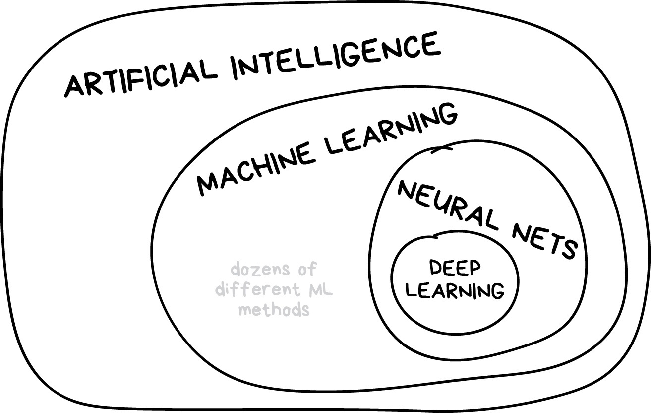
• The goal of machine learning is use input data to make useful predictions on never-before-seen data

• Machine learning is part of artificial intelligence, but not the only part

Input data

• Machine learning starts with a labelled dataset

• A label (or target variable) is the thing we're predicting (e.g. y variable in linear regression)

• For example, house price, river discharge, land cover etc.

Input data

• It's tough to collect a good collection of data (time-consuming, expensive)

• These datasets are therefore extremely valuable

Features

• An input variable (e.g. the x variable in linear regression)

• A simple dataset might use a one or two features while a more complex dataset could have thousands of features

• In our river discharge example - features could include precipitation, snow depth, soil moisture

Algorithms

• There are many (e.g. naive bayes, decision trees, neural network etc.)

• Performance of algorithm dependent on type of problem

• Just remember: garage in, garbage out

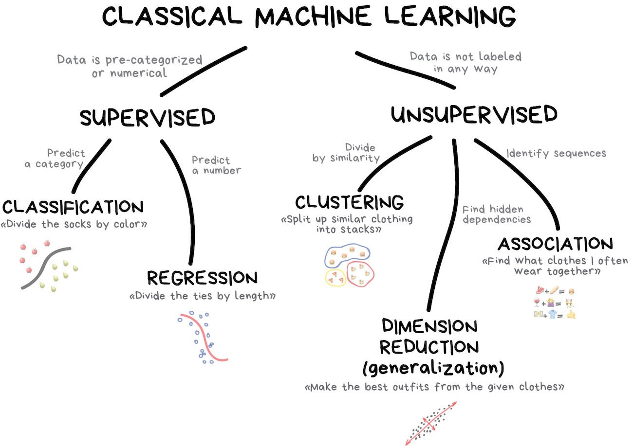
Supervised learning

• Training data is already labeled and we teach the machine to learn from these examples

• Supervised learning can used to predict a category (classification) or predict a number (regression)

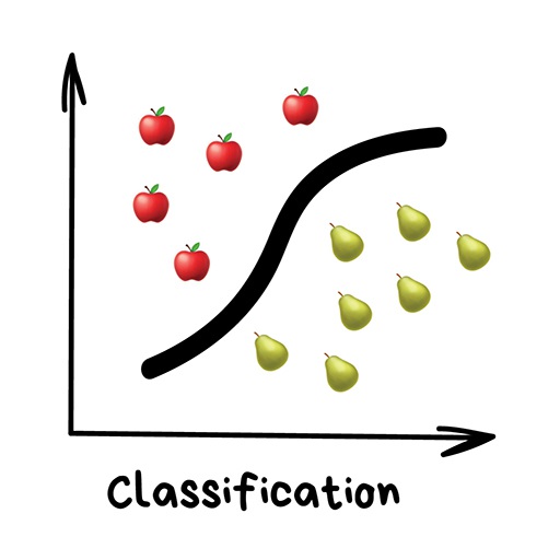
Classification

• "Split things into groups based on their features"

• Examples include:

  • Land cover
  • Flood risk
  • Sentiment analysis

• Popular algorithms include:

  • Naive Bayes
  • Decision Trees
  • K-Nearest Neighbours
  • Support Vector Machine

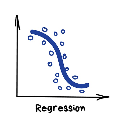
Regression

• "Draw a line through these dots"

• Used for predicting continuous variables:

  • River discharge
  • House prices
  • Weather forecasting

• Popular algorithms include linear regression, polynomial regression, + other algorithms

Unsupervised learning

• Labeled data is a luxury, sometimes we don't have it

• Sometimes we have no idea what the labels could be

• Much less used in geospatial data science but sometimes useful for exploratory analysis

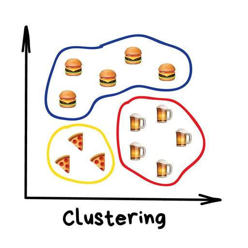
Clustering

• "Divide data into groups but machine chooses the best way"

• Common usages include:

  • image compression
  • labeling training data (i.e. for supervised learning)
  • detecting abnormal behavior

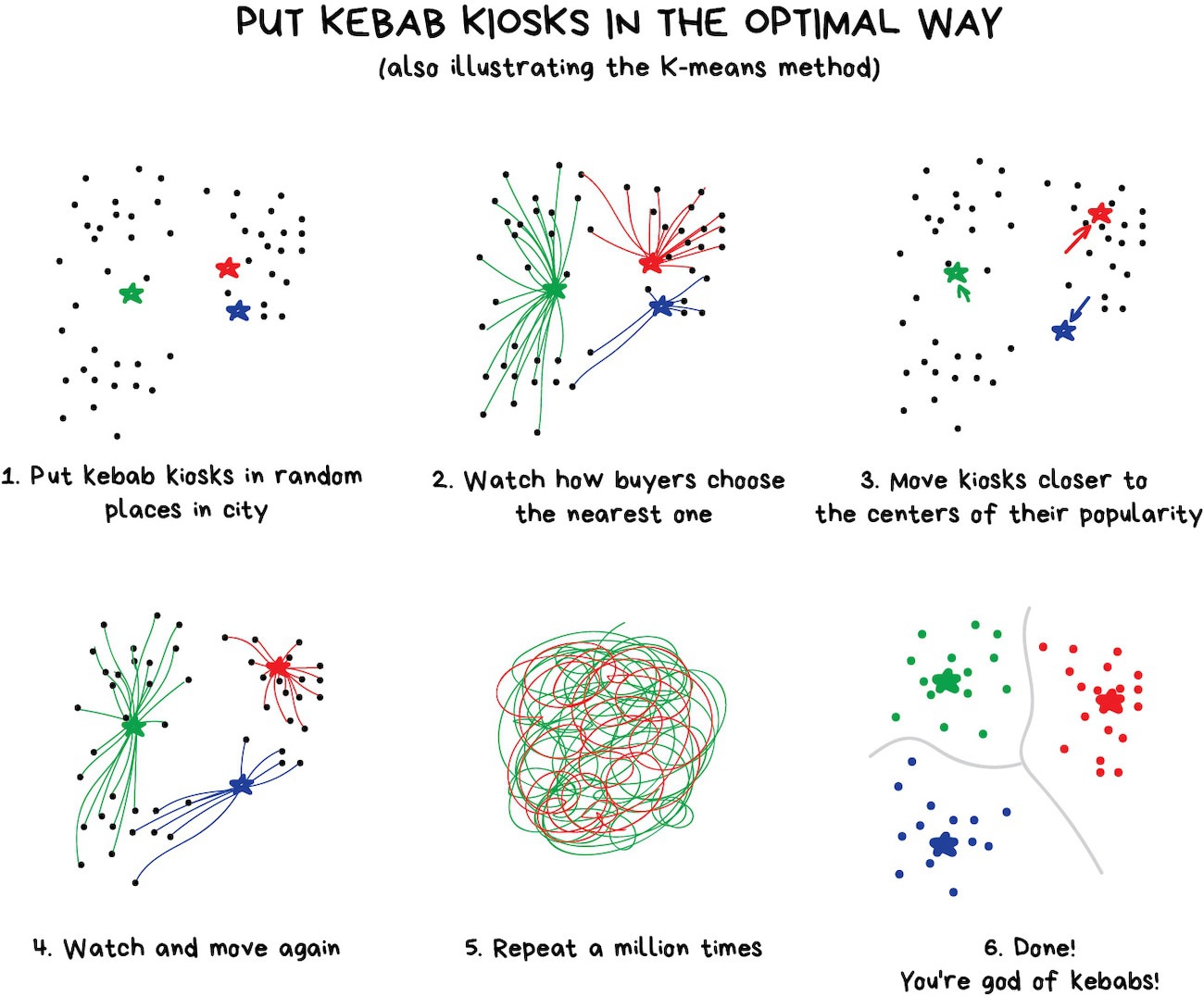
• Popular algorithms:

  • K-means clustering
  • Mean-Shift
  • DBSCAN

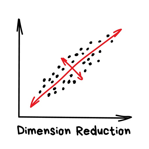
Dimensionality reduction

• "Assemble specific features into higher-level ones"

• When we have too many features, some of which are useless

• Most popular algorithm is Principal Component Analysis (PCA)

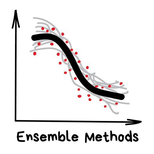
Ensemble methods

• "Multiple learning algorithms learning to correct errors of each other"

• Often used improve the accuracy over what could be acheived with a single classical machine learning model.

• Popular algorithms:

  • Random Forest
  • XGBoost

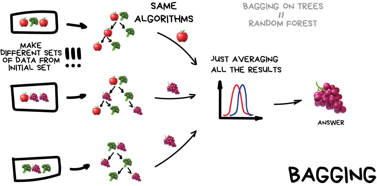
Bagging

• Apply the same algorithm but train it on different subsets of original data. At the end - just average the answers. Most famous example is Random Forests.

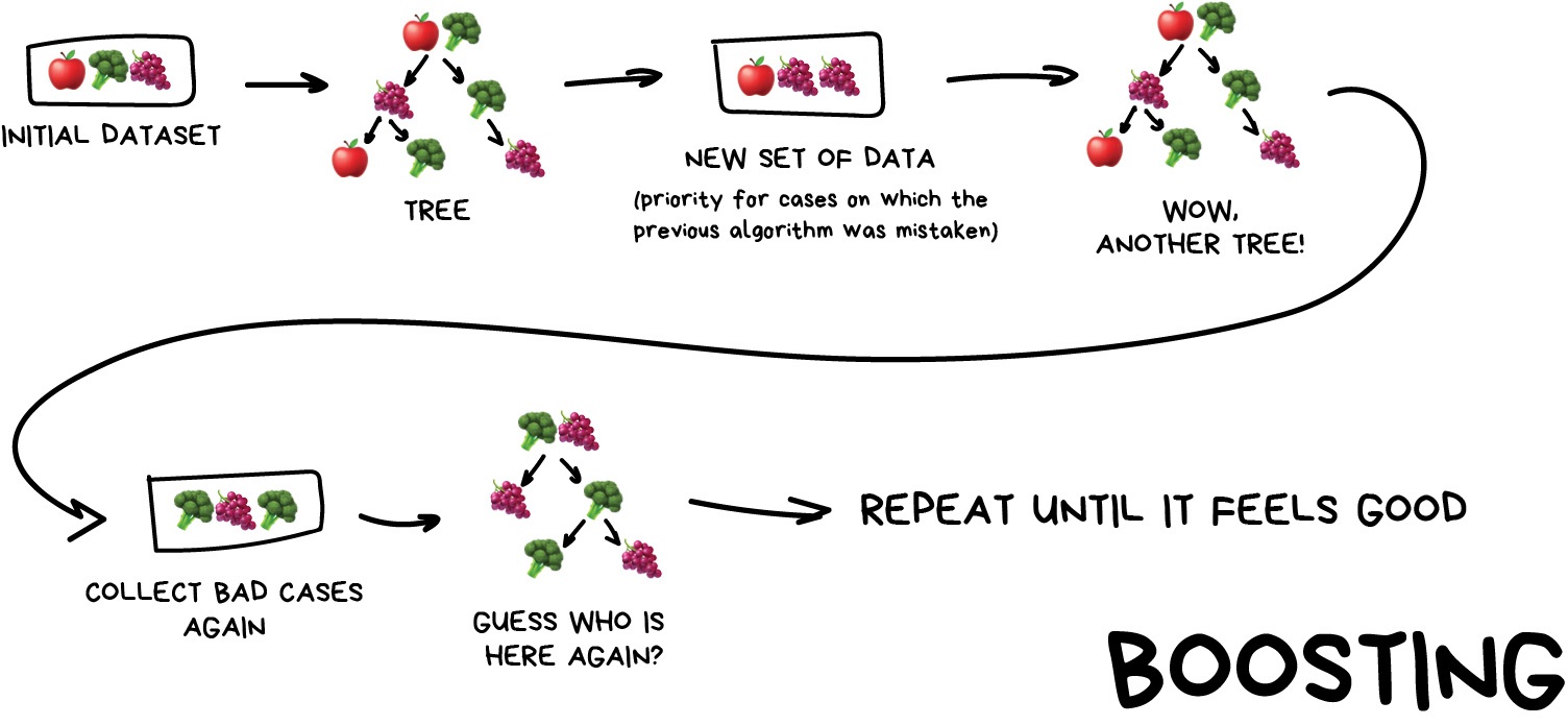
Boosting

Similar to bagging but each subsequent algorithm is paying most attention to data points that were mispredicted by the previous one.

Predicting house prices using scikit-learn

• The California house price dataset is a classic example dataset derived from the 1990 U.S. Census

• Labels = house prices at the block group level (a block group typically has a population of 600 to 3,000 people)

• Features = longitude, latitude, housing_median_age, total_rooms, total_bedrooms, population, households, median_income

# Import libraries
import pandas as pd
import numpy as np
import matplotlib.pyplot as plt

# Read dataset
df = pd.read_csv('data/california_house_prices.csv')

# Examine dataset (each row represents one block group)
df.head()

	housing_median_age	total_rooms	total_bedrooms	population	households	median_income	median_house_value
0	51	1905	291	707	284	6.2561	431000
1	51	1616	374	608	302	3.1932	400000
2	51	2413	431	1095	437	4.0089	357000
3	51	1502	243	586	231	4.3750	332400
4	51	2399	516	1160	514	3.8456	318900

Check data

# Check for NaN values and data types
df.info()

<class 'pandas.core.frame.DataFrame'>
RangeIndex: 15267 entries, 0 to 15266
Data columns (total 7 columns):
 #   Column              Non-Null Count  Dtype  
---  ------              --------------  -----  
 0   housing_median_age  15267 non-null  int64  
 1   total_rooms         15267 non-null  int64  
 2   total_bedrooms      15267 non-null  int64  
 3   population          15267 non-null  int64  
 4   households          15267 non-null  int64  
 5   median_income       15267 non-null  float64
 6   median_house_value  15267 non-null  int64  
dtypes: float64(1), int64(6)
memory usage: 835.0 KB

Check data

# Check summary statistics
df.describe()

	housing_median_age	total_rooms	total_bedrooms	population	households	median_income	median_house_value
count	15267.000000	15267.000000	15267.000000	15267.000000	15267.000000	15267.00000	15267.000000
mean	26.924805	2678.617214	549.977075	1476.071199	510.814371	3.70112	189416.617345
std	11.426288	2225.565198	430.964703	1180.890618	393.232807	1.57686	95681.349164
min	1.000000	2.000000	2.000000	3.000000	2.000000	0.49990	14999.000000
25%	17.000000	1469.000000	302.000000	814.000000	286.000000	2.53665	115400.000000
50%	27.000000	2142.000000	441.000000	1203.000000	415.000000	3.47840	171200.000000
75%	36.000000	3187.000000	661.000000	1780.000000	614.500000	4.62635	243050.000000
max	51.000000	37937.000000	6445.000000	35682.000000	6082.000000	15.00010	499100.000000

Visualize data

# Plot histogram
_ = df.hist(bins=50 , figsize=(20, 10))

Correlation analysis

• It is always useful to compute correlation coeffcients (e.g.Pearson's r) between the labels (i.e. median_house_value) and features.

# Compute correlation matrix
corr_matrix = df.corr()

# Display just house value correlations
corr_matrix["median_house_value"].sort_values(ascending= False)

median_house_value    1.000000
median_income         0.668566
total_rooms           0.152923
households            0.098525
total_bedrooms        0.079023
population            0.020930
housing_median_age    0.014355
Name: median_house_value, dtype: float64

Warning

• Just remember that correlation coefficients only measure linear correlations ("if x goes up, then y generally goes up/down").

• They may completely miss nonlinear relationships (e.g., "if x is close to zero then y generally goes up").

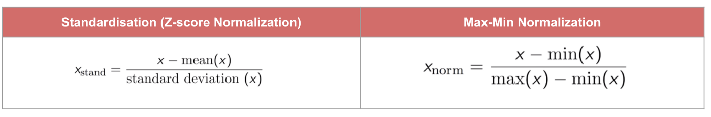
Feature scaling

• Machine Learning algorithms don’t perform well when the input numerical attributes have very different scales.

• We often scale (or normalize) our features before training the model (e.g. min-max scaling or standardization).

• Min-max method scales values so that they end up ranging from 0 to 1

• Standardization scales values so that the they have mean of 0 and unit variance.

# Import library
from sklearn.preprocessing import StandardScaler

# Define feature list
feature_list =  ['housing_median_age', 'total_rooms', 'total_bedrooms', 
                 'population', 'households', 'median_income']

# Define features and labels 
X = df[feature_list]
y = df['median_house_value']

# Standarize data
scaler = StandardScaler()  
X_scaled = scaler.fit_transform(X)

Split data in training and testing subsets

from sklearn.model_selection import train_test_split

# Split data 
X_train, X_test, y_train, y_test = train_test_split(X_scaled, y, test_size=0.2, random_state=42)

Multiple linear regression

A very simple supervised algorithm that fits a linear model to our data using a least squares approach.

from sklearn.linear_model import LinearRegression

# Define model
lin_reg = LinearRegression()

# Fit model to data
lin_reg.fit(X_train, y_train)

LinearRegression()

from sklearn.metrics import mean_squared_error

# Predict test labels
predictions = lin_reg.predict(X_test)

# Compute mean-squared-error
lin_mse = mean_squared_error(y_test, predictions)
lin_rmse = np.sqrt(lin_mse)
lin_rmse

64374.61617631897

# Plot
fig, ax = plt.subplots(figsize=(8, 6))
ax.scatter(y_test, predictions, alpha=0.1, s=50, zorder=2)
ax.plot([0,500000], [0, 500000], color='k', lw=1, zorder=3)
ax.set_ylabel('Predicted house price ($)', fontsize=14)
ax.set_xlabel('Observed house price ($)', fontsize=14)
ax.tick_params(axis='both', which='major', labelsize=13)
ax.grid(ls='dashed', lw=1, zorder=1)
ax.set_ylim(0,500000)
ax.set_xlim(0,500000)

(0.0, 500000.0)

Decision Tree

A popular machine learning algorithm that predicts a target variable using multiple regression trees

from sklearn.tree import DecisionTreeRegressor

# Define model
tree_reg = DecisionTreeRegressor()

# Fit model
tree_reg.fit(X_train, y_train)

DecisionTreeRegressor()

# Predict test labels
predictions = tree_reg.predict(X_test)

# Compute mean-squared-error
tree_mse = mean_squared_error(y_test, predictions)
tree_rmse = np.sqrt(tree_mse)
tree_rmse

82289.76594673106

# Plot
fig, ax = plt.subplots(figsize=(8, 6))
ax.scatter(y_test, predictions, alpha=0.1, s=50, zorder=2)
ax.plot([0,500000], [0, 500000], color='k', lw=1, zorder=3)
ax.set_ylabel('Predicted house price ($)', fontsize=14)
ax.set_xlabel('Observed house price ($)', fontsize=14)
ax.tick_params(axis='both', which='major', labelsize=13)
ax.grid(ls='dashed', lw=1, zorder=1)
ax.set_ylim(0,500000)
ax.set_xlim(0,500000)

(0.0, 500000.0)

RandomForests

A popular ensemble algorithm that fits a number of decision tree classifiers on various sub-samples of the dataset and uses averaging to improve the predictive accuracy and control over-fitting.

from sklearn.ensemble import RandomForestRegressor

# Define model
forest_reg = RandomForestRegressor(n_estimators = 30)

# Fit model
forest_reg.fit(X_train, y_train)

RandomForestRegressor(n_estimators=30)

# Predict test labels predictions
predictions = forest_reg.predict(X_test)

# Compute mean-squared-error
final_mse = mean_squared_error(y_test , predictions)
final_rmse = np.sqrt(final_mse)
final_rmse

60264.63679436083

# Plot
fig, ax = plt.subplots(figsize=(8, 6))
ax.scatter(y_test, predictions, alpha=0.1, s=50, zorder=2)
ax.plot([0,500000], [0, 500000], color='k', lw=1, zorder=3)
ax.set_ylabel('Predicted house price ($)', fontsize=14)
ax.set_xlabel('Observed house price ($)', fontsize=14)
ax.tick_params(axis='both', which='major', labelsize=13)
ax.grid(ls='dashed', lw=1, zorder=1)
ax.set_ylim(0,500000)
ax.set_xlim(0,500000)

(0.0, 500000.0)