Today's Talk
- My project
- Black-box function approximation
- Deterministic approach: Neural networks and Long-short term memory (LSTMs)
- Probabilistic approach: Gaussian processes (GPs)
- Timeseries applications
- Key takeaways
1. My Project

Video: Deepmind's Deep Q-network solving the Atari game Breakout after 600 episodes of self-play (Mnih et. al (2013))


Figure: Top:* AlphaGo's infamous Move 37, a counterintuitive move for a human to make with this board set-up, but nonetheless a gaming-winning one. Bottom: Lee Sedol, the world no.1 Go player, flumexed by AlphaGo's moves. (Silver et al (2017))*

Figure: The complex, interconnected electricity grid
1.1 Reinforcement Learning

Figure: The RL control loop. Agent's take sequential actions that affect their environment, the environment changes and the agent receives a reward for their action. Adapted from Episode 1 of David Silver's RL Youtube series
More formally, the RL control loop looks something like this:
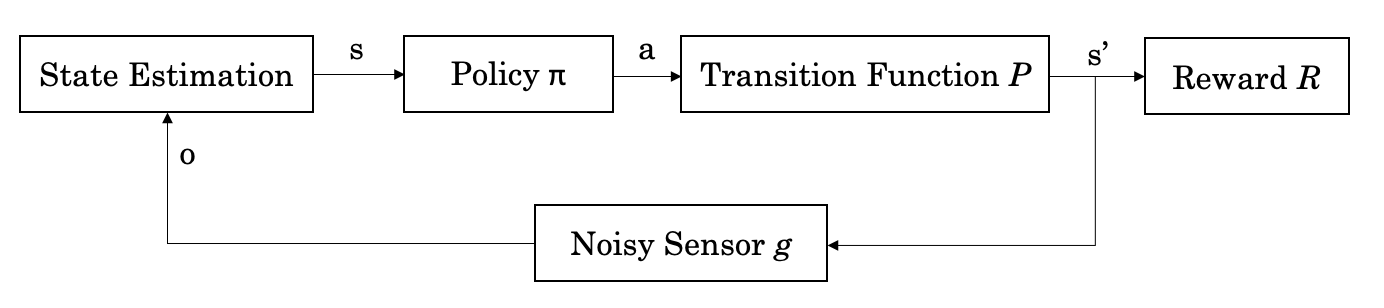
Figure: The formalised RL control loop.
2. Black-box Function Approximation
2.1 Two approaches to modelling
Generally when we model a function using a black-box approximator, we can select (informally) from two sets of models, these are:
- Deterministic models: Do not contain elements of randomness; everytime the model is run with the same initial conditions it produces identical results.
- Probabilistic models: Include elements of randomness; trials with identical initial conditions will produce different results.
2.2 Deterministic Models: Neural Networks

Linear Basis
$$ f(x) = {\color{red}{w_0}} + {\color{blue}{w_1} x} $$from ipywidgets import interact
import ipywidgets as widgets
def y_linear_plot(w1, w0):
y_lin = w1*x_true+w0
y_err = w1*x+w0
with plt.xkcd():
fig = plt.figure(figsize=(10,5))
plt.xlim([-6,6])
plt.ylim([-4,4])
plt.scatter(x, y, 100, 'k', 'o', zorder=100)
plt.plot(x_true, y_lin)
plt.vlines(x=x, ymin=y_err, ymax=y, colors='green', ls=':', lw=2)
plt.savefig(path+'/images/2_data.png', dpi=300)
plt.show()
interact(y_linear_plot, w1=widgets.FloatSlider(value=0.75, min=-5, max=5, step=0.25),
w0=widgets.FloatSlider(value=-.25, min=-5, max=5, step=0.25))
interactive(children=(FloatSlider(value=0.75, description='w1', max=5.0, min=-5.0, step=0.25), FloatSlider(val…
<function __main__.y_linear_plot(w1, w0)>
Polynomial Basis
$$ f(x) = {\color{red}{w_0}} + {\color{blue}{w_1}} x + {\color{green}{w_2}} x^2 + {\color{orange}{w_3}} x^3 $$def y_poly_plot(w0, w1, w2, w3):
y_poly = w0 + w1*x_true + w2*(x_true**2) + w3*(x_true**3)
y_polyerr = w0 + w1*x + w2*(x**2) + w3*(x**3)
with plt.xkcd():
fig = plt.figure(figsize=(10,5))
plt.xlim([-6,6])
plt.ylim([-4,4])
plt.scatter(x, y, 100, 'k', 'o', zorder=100)
plt.plot(x_true, y_poly)
plt.vlines(x=x, ymin=y_polyerr, ymax=y, colors='green', ls=':', lw=2)
plt.savefig(path+'/images/3_data.png', dpi=300)
plt.show()
interact(y_poly_plot,
w0=widgets.FloatSlider(value=-1, min=-7, max=7, step=0.5),
w1=widgets.FloatSlider(value=-.5, min=-7, max=7, step=0.5),
w2=widgets.FloatSlider(value=1.5, min=-7, max=7, step=0.5),
w3=widgets.FloatSlider(value=1, min=-7, max=7, step=0.5),
)
interactive(children=(FloatSlider(value=-1.0, description='w0', max=7.0, min=-7.0, step=0.5), FloatSlider(valu…
<function __main__.y_poly_plot(w0, w1, w2, w3)>
Rectified Linear Unit (ReLU)
$$ f(x) = \max (0 , {\color{blue}{w_1}} x + {\color{red}{w_0}}) $$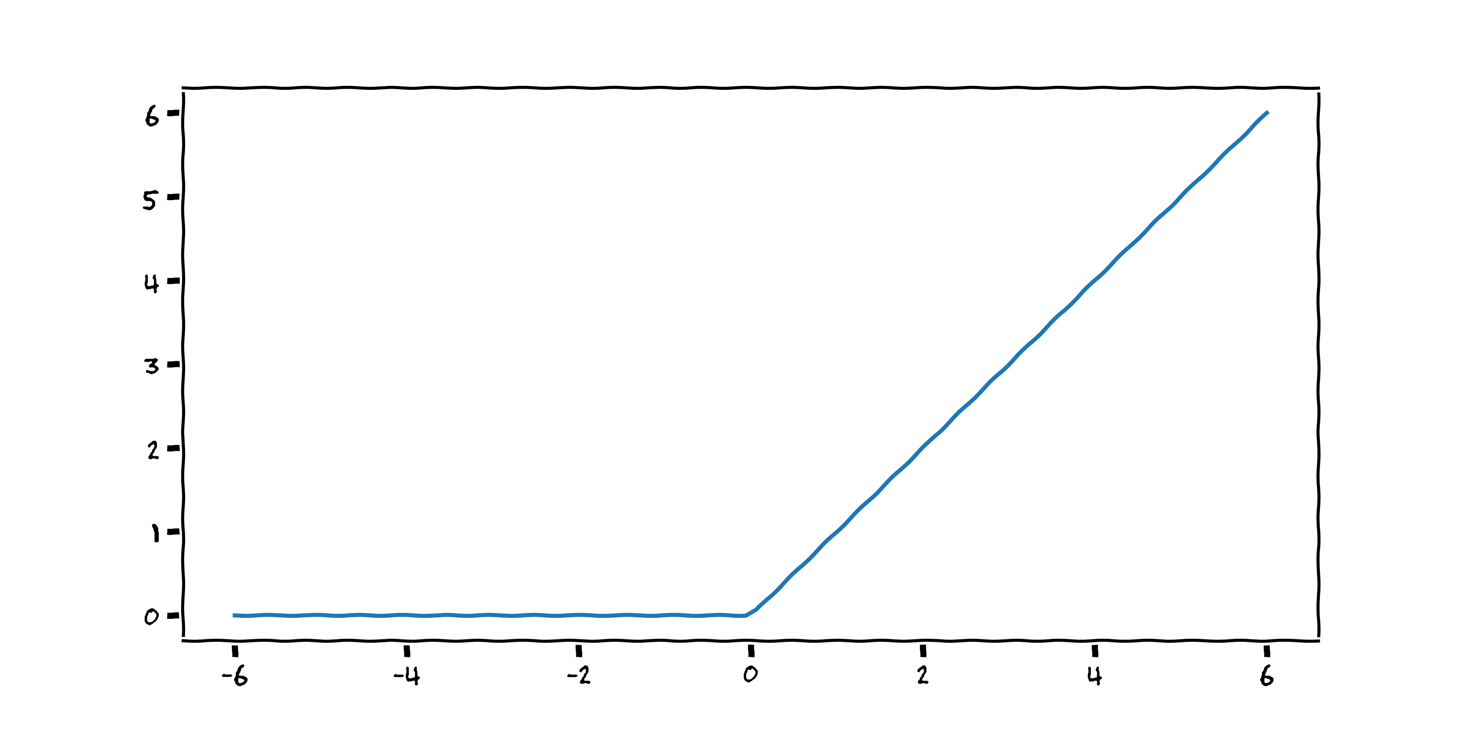
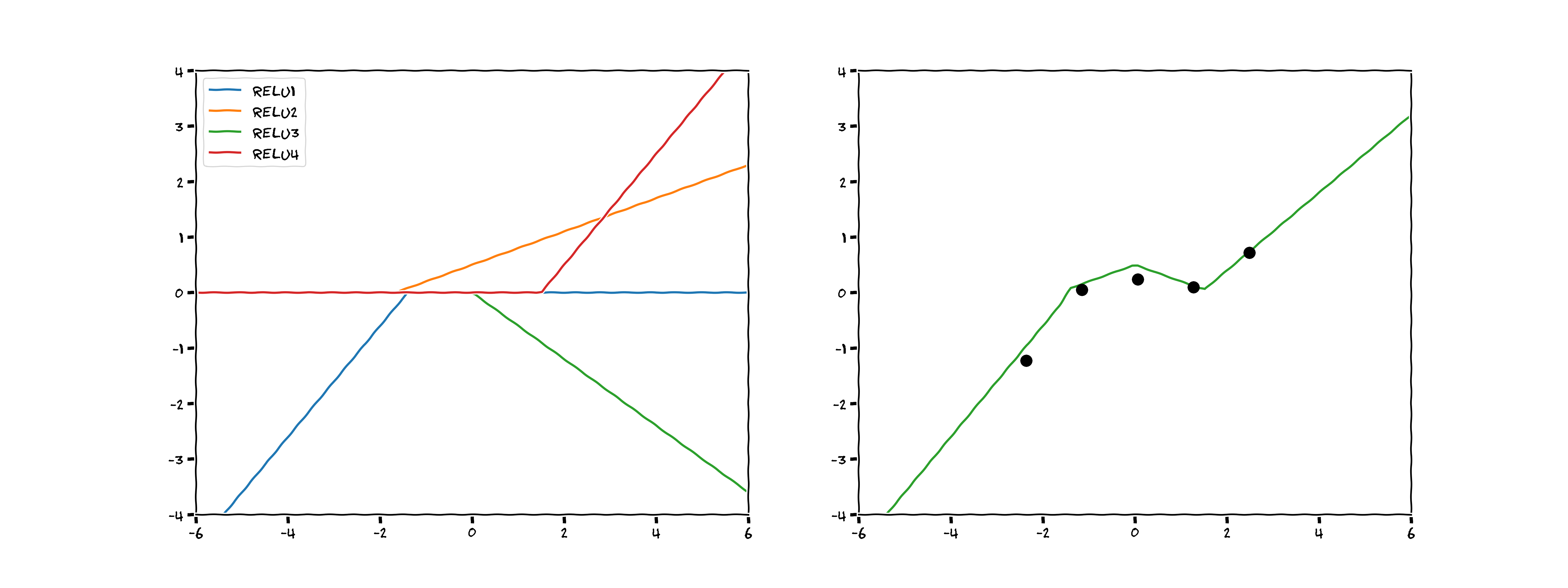


Figure: Top:* A neural network with 4 nodes and 1 hidden layer–a graph of the model created by hand above. Bottom: A neural network with 10 nodes and 2 hidden layers–a more typical model arrangement.*


3. Probabilistic Models: Gaussian Processes
We use Bayes' rule to narrow the solution space, which tells us how to update our beliefs about the world based on the evidence we've seen:
$$ P (A | B) = \frac{P(B | A) P(A)}{P(B)} $$and in the setting of functions and data it looks something like:
$$ P (\textbf{f} | \textbf{D}) = \frac{P(\textbf{D} | \textbf{f}) P(\textbf{f})}{P(\textbf{D})} $$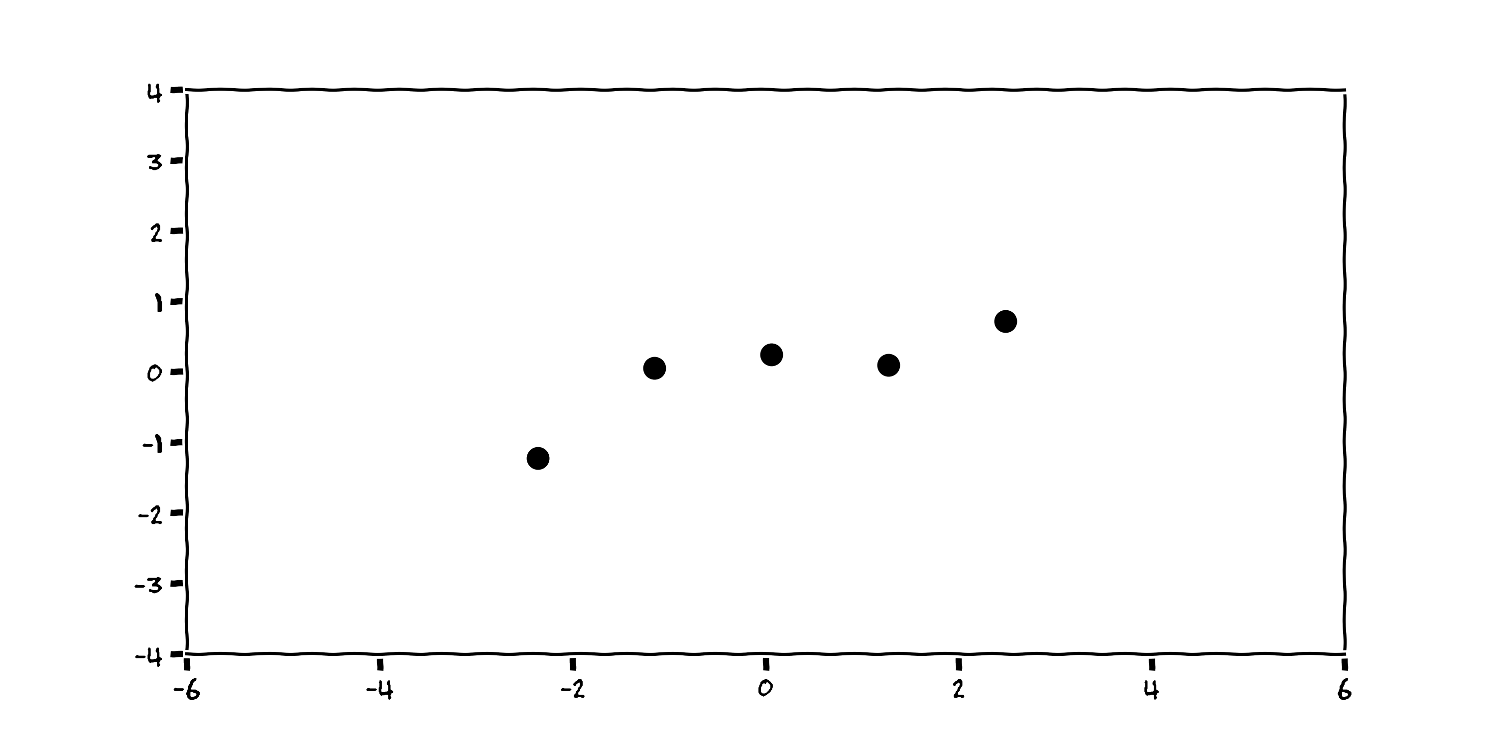
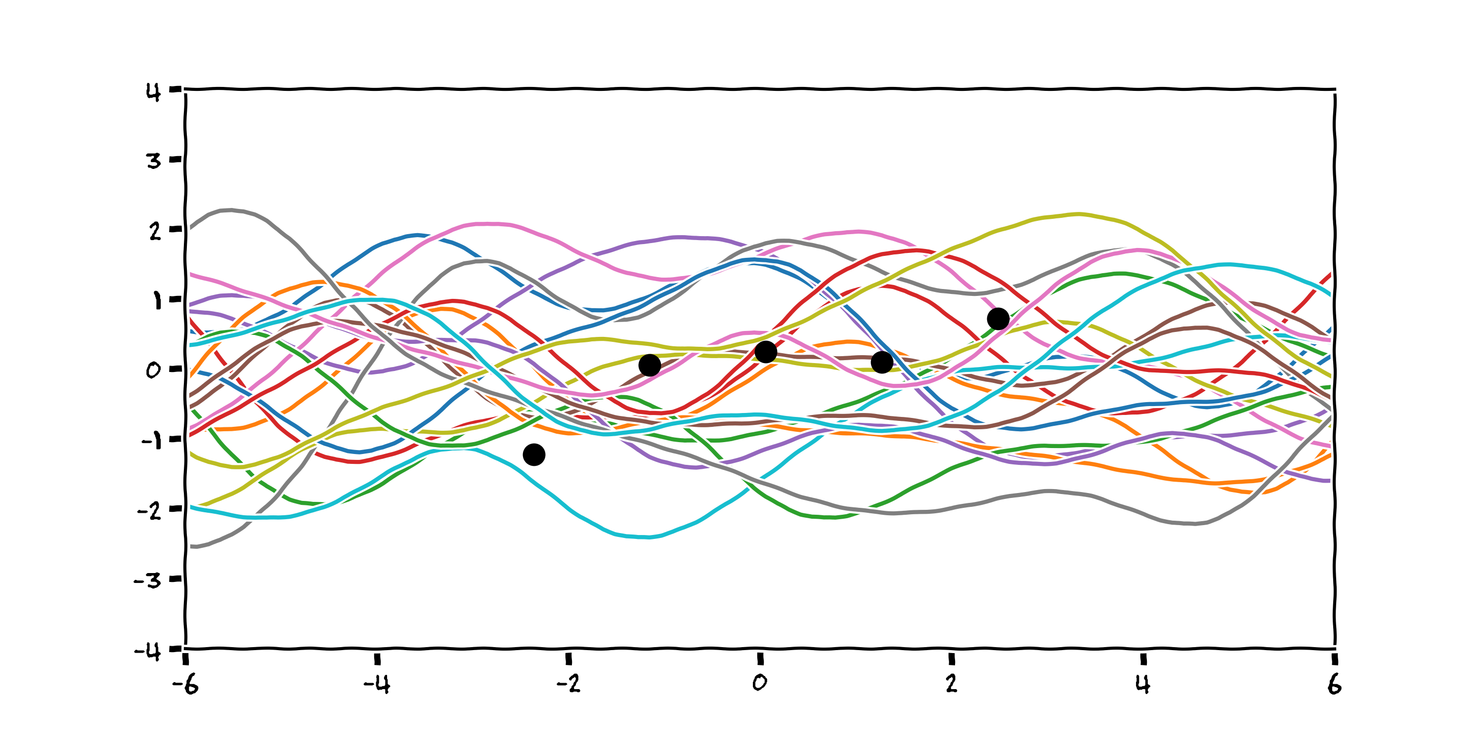
# plot rbf kernel
with plt.xkcd():
    fig = plt.figure(figsize=(10,5))
    plt.scatter(x, y, 100, 'k', 'o', zorder=100)
    plt.plot(x_true, f_rbf.T)
    plt.xlim([-6,6])
    plt.ylim([-4,4])
    plt.savefig(path+'/images/8_data.png', dpi=300)
    plt.show()

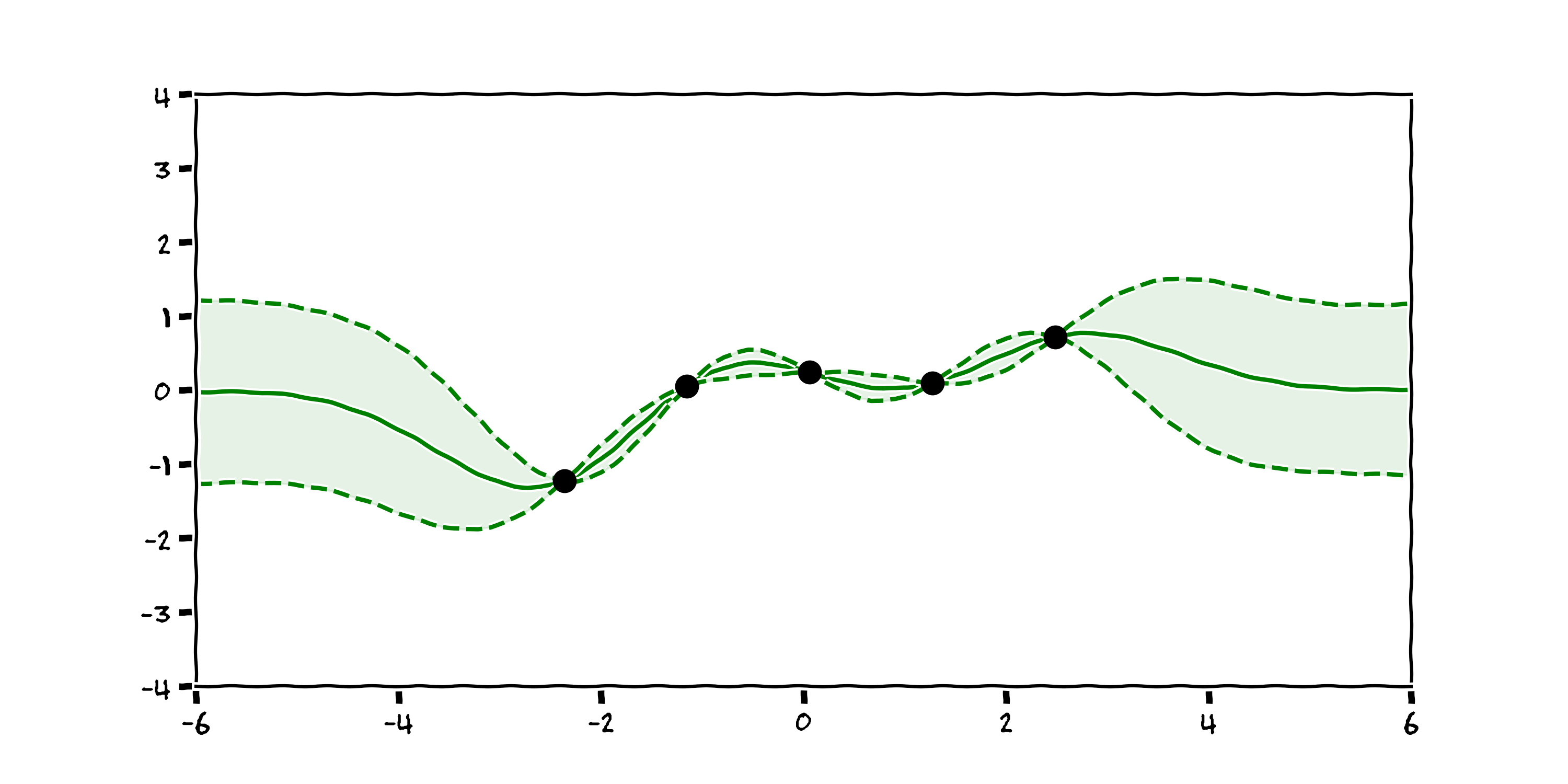
3.1 Prior Beliefs
3.2 (Different) Prior Beliefs


3.3 Drawbacks
- Expensive to compute; N > ~50,000 prohibitively large
- Prior knowledge remains crucial
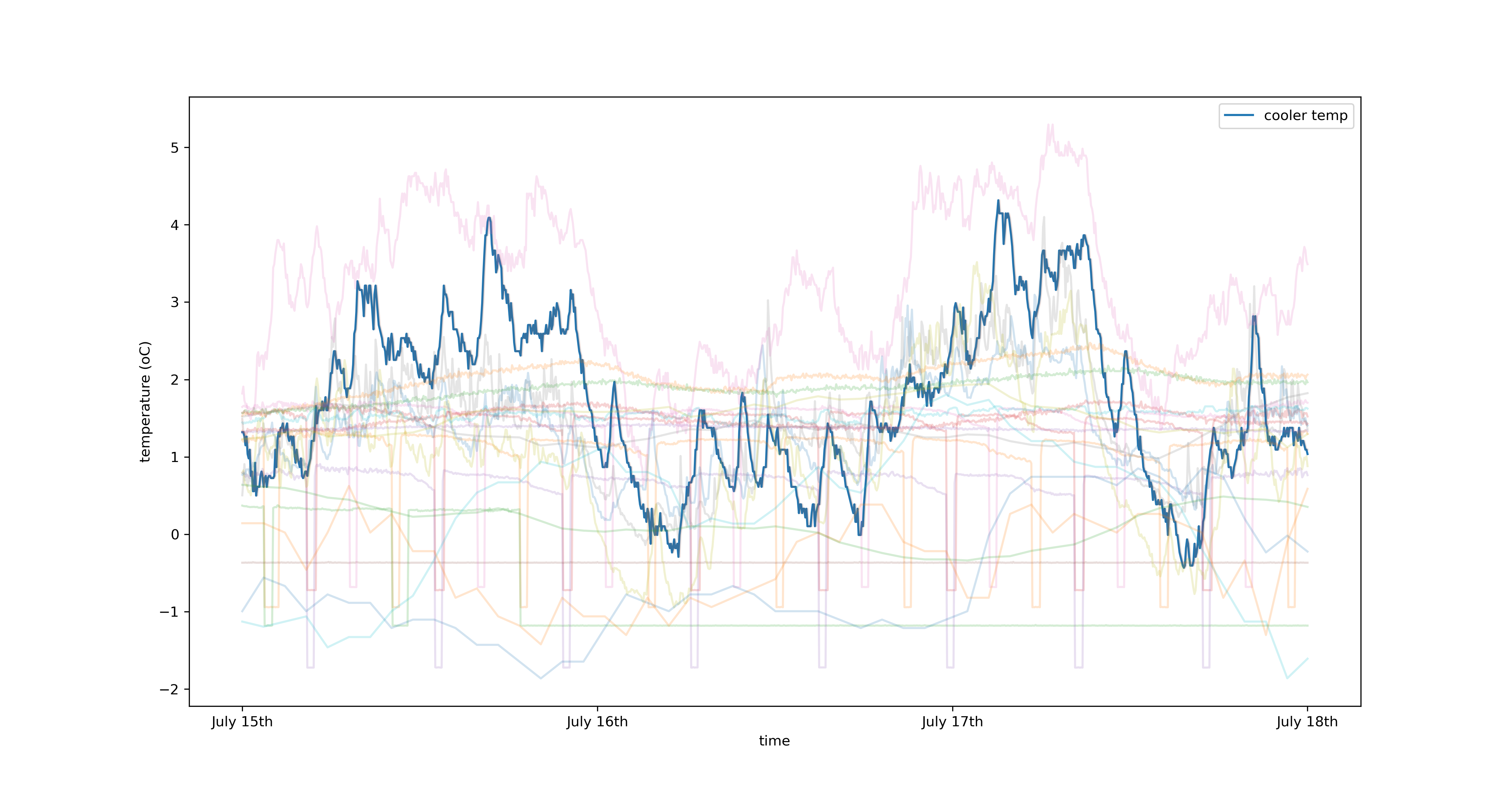
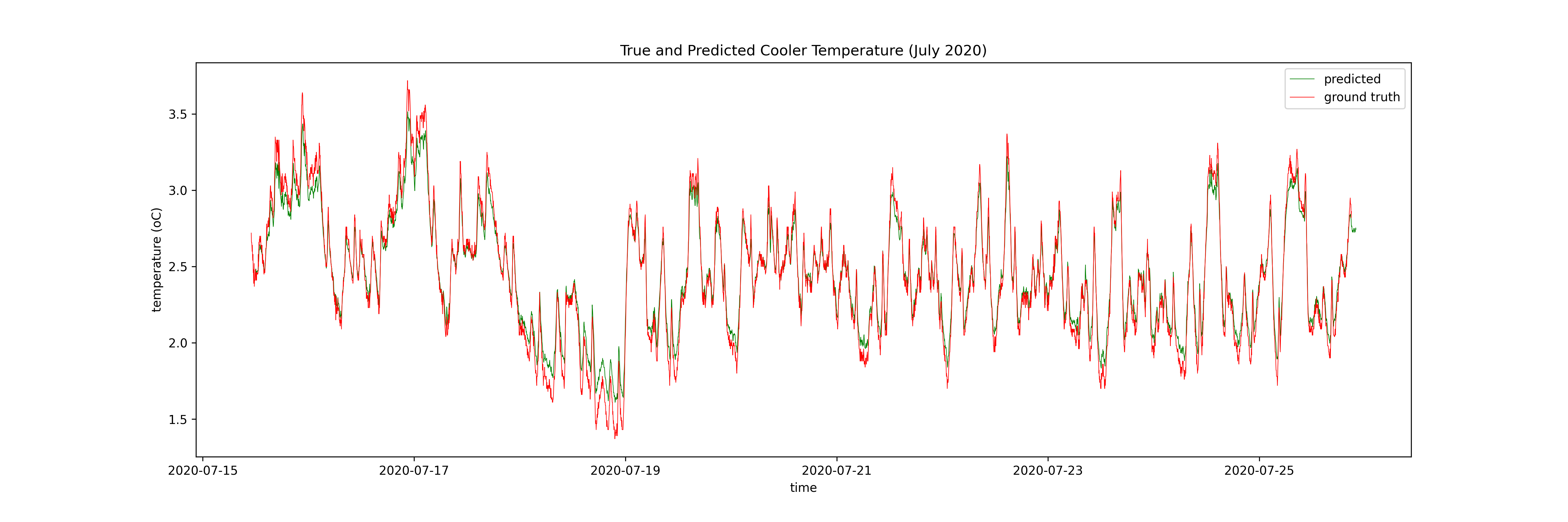
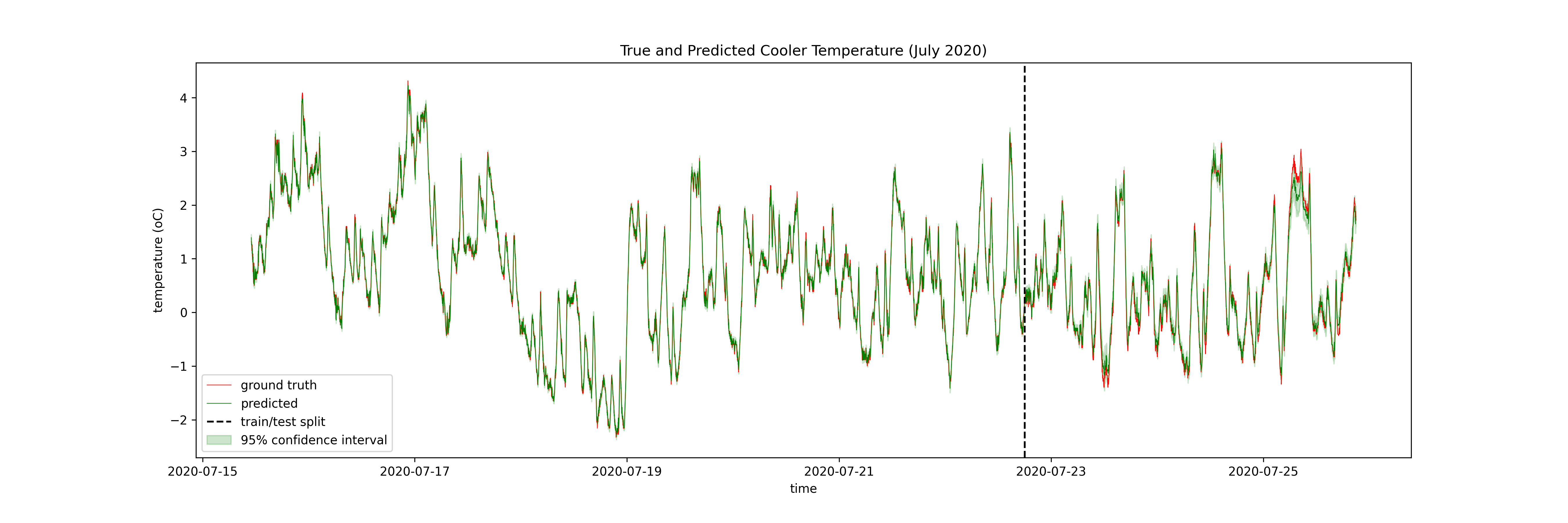
4. Timeseries Applications

5. Key Takeaways
- Black box function approximators can model any continuous function in theory
- Deterministic techniques effective with large (N > $10^5$) datasets
- Probabilistic techniques more robust in low data regimes thanks to uncertainty quantification
- GPs are limited by their expensive computations (N must be < $10^5$)
- Both approaches can be used to model complex timeseries datasets
Further Reading
Further explanations on why these techniques work
How can you build these in practice?
- Neural nets: Introduction to deep learning with tensorflow
- GPs: GP regression on molecules
- LSTMs: LSTMs for timeseries prediction
Introductory Books
Thanks!
- Notes: https://enjeeneer.io/talks/2021-03-15-xchangeseminar/
- Thanks to Carl Henrik Ek, Dept. of Computer Science for inspiring these slides
- Questions?