Start with Python
Python installation
PythonXY https://code.google.com/p/pythonxy/
WinPython http://winpython.github.io/
Anaconda https://store.continuum.io/cshop/anaconda/
Programming in Python http://pythonic.eu/fjfi/
Web page of Image Processing course http://www.kky.zcu.cz/cs/courses/zdo
Demo of image processing http://scipy-lectures.github.io/packages/scikit-image/
Run notebook
- Jupyter notebook cells
- Run cell:
Ctrl-Enter
In [1]:
%pylab inline

# from pylab import *
# import cStringIO
import urllib
import scipy
import scipy.misc
import skimage
import skimage.data
from skimage.filters import threshold_otsu
# from skimage.filters import gaussian_filter
from skimage.filters import gaussian as gaussian_filter
# from skimage.filter import threshold_otsu, gaussian_filter
from skimage.morphology import label
from scipy.ndimage.morphology import binary_closing, binary_erosion, binary_opening, binary_dilation

from skimage.measure import regionprops
from skimage.color import label2rgb
from skimage.io import imread
# import skimage.filter
# from skimage.filters import
Populating the interactive namespace from numpy and matplotlib
In [ ]:
Little bit of python
In [2]:
print("hello")
hello
In [13]:
def myFunction(vstup):
    vystup = vstup + 6
    return vystup

myFunction(5)
Out[13]:
11
In [4]:
for i in range(2,5):
    print(i)
2
3
4
In [14]:
pole = ['Franta', 'Jakub', 'Marta']

for jmeno in pole:
    print(jmeno)
Franta
Jakub
Marta
Image Processing in Python
Read image from URL
In [6]:
URL = "http://plzen.cz/cameraFeed.php"
img = imread(URL)

imshow(img)
# show()
Out[6]:
<matplotlib.image.AxesImage at 0x2056520efd0>

Colors
In [7]:
plt.figure(figsize=[10, 5])
subplot(131)
imshow(img[:, :, 0], cmap="Reds")
plt.axis("off")
subplot(132)
imshow(img[:, :, 1], cmap="Greens")
plt.axis("off")
subplot(133)
imshow(img[:, :, 2], cmap="Blues")
plt.axis("off")
img.shape
Out[7]:
(960, 1280, 3)

Read gray image from file or URL
In [15]:
# URL = "http://uc452cam01-kky.fav.zcu.cz/snapshot.jpg"
URL = "https://github.com/mjirik/ZDO/raw/master/objekty/dataset/01.jpg"
In [11]:
img = imread(URL, as_grey=True)
imshow(img, cmap='gray')
Out[11]:
<matplotlib.image.AxesImage at 0x20566938128>

In [16]:
# ukazkova data
img = skimage.data.coins() / 255.0
imshow(img, cmap='gray')
Out[16]:
<matplotlib.image.AxesImage at 0x205667484e0>

Manipulation with image data
In [17]:
img.shape
Out[17]:
(303, 384)
In [18]:
img[50, 10]
Out[18]:
0.43529411764705883
In [19]:
imgi = img.astype(np.int)
imgi
Out[19]:
array([[0, 0, 0, ..., 0, 0, 0],
       [0, 0, 0, ..., 0, 0, 0],
       [0, 0, 0, ..., 0, 0, 0],
       ...,
       [0, 0, 0, ..., 0, 0, 0],
       [0, 0, 0, ..., 0, 0, 0],
       [0, 0, 0, ..., 0, 0, 0]])
In [20]:
img[10:20,15:20]
Out[20]:
array([[ 0.49411765,  0.48627451,  0.49411765,  0.50196078,  0.50588235],
       [ 0.49411765,  0.4745098 ,  0.4745098 ,  0.48627451,  0.49411765],
       [ 0.49019608,  0.49411765,  0.48627451,  0.48627451,  0.49019608],
       [ 0.48627451,  0.49803922,  0.48627451,  0.48235294,  0.49019608],
       [ 0.47843137,  0.47843137,  0.47843137,  0.48235294,  0.49019608],
       [ 0.4745098 ,  0.48235294,  0.48627451,  0.49411765,  0.49411765],
       [ 0.48627451,  0.47843137,  0.48235294,  0.48627451,  0.48627451],
       [ 0.48627451,  0.4745098 ,  0.47843137,  0.48235294,  0.48627451],
       [ 0.48627451,  0.47843137,  0.47843137,  0.48235294,  0.48235294],
       [ 0.47843137,  0.47843137,  0.48235294,  0.48235294,  0.48235294]])
In [21]:
# img[10:200, 10:-100] = 100
imshow(img, cmap='gray')
colorbar()
Out[21]:
<matplotlib.colorbar.Colorbar at 0x205667e0080>

In [40]:
imshow(img[100:200, 100:200], cmap="gray")
Out[40]:
<matplotlib.image.AxesImage at 0x20568fa0f60>

Segmentace
In [22]:
imthr = img > 0.2
imshow(imthr, cmap='gray')
Out[22]:
<matplotlib.image.AxesImage at 0x2056685b860>

In [23]:
imthr = img > 0.50
imshow(imthr, cmap='gray')
Out[23]:
<matplotlib.image.AxesImage at 0x205668c0208>

In [ ]:
Image labeling
In [24]:
# blobs_labels = skimage.morphology.label(img, background=0)
imlabel = label(imthr, background=0)
imshow(imlabel, cmap='gray')
Out[24]:
<matplotlib.image.AxesImage at 0x205675fcf98>

In [25]:
np.unique(imlabel)
Out[25]:
array([  0,   1,   2,   3,   4,   5,   6,   7,   8,   9,  10,  11,  12,
        13,  14,  15,  16,  17,  18,  19,  20,  21,  22,  23,  24,  25,
        26,  27,  28,  29,  30,  31,  32,  33,  34,  35,  36,  37,  38,
        39,  40,  41,  42,  43,  44,  45,  46,  47,  48,  49,  50,  51,
        52,  53,  54,  55,  56,  57,  58,  59,  60,  61,  62,  63,  64,
        65,  66,  67,  68,  69,  70,  71,  72,  73,  74,  75,  76,  77,
        78,  79,  80,  81,  82,  83,  84,  85,  86,  87,  88,  89,  90,
        91,  92,  93,  94,  95,  96,  97,  98,  99, 100, 101, 102, 103,
       104, 105, 106, 107, 108, 109, 110, 111, 112, 113, 114, 115, 116,
       117, 118, 119], dtype=int64)
In [26]:
# pocet labelu
print(np.max(imlabel))
119
Zobrazení jednoho objektu
In [27]:
imshow(imlabel==35)
Out[27]:
<matplotlib.image.AxesImage at 0x2056766c358>

In [28]:
fig, axes = subplots(1,3, figsize=(15,4))
axes[0].imshow(imlabel==35)
axes[1].imshow(imlabel==36)
axes[2].imshow(imlabel==64)
Out[28]:
<matplotlib.image.AxesImage at 0x205677264a8>

Color visualization of labeling
In [29]:
# Barevne provedeni
image_label_overlay = label2rgb(imlabel, image=img)
plt.imshow(image_label_overlay)
Out[29]:
<matplotlib.image.AxesImage at 0x2056776d5f8>

Filtration
In [30]:
coins_zoom = img[10:80, 300:370]
from scipy import ndimage
gaussian_coins1 = gaussian_filter(coins_zoom, sigma=1)
gaussian_coins2 = gaussian_filter(coins_zoom, sigma=15)

fig, axes = subplots(1,3, figsize=(15,4))
axes[0].imshow(coins_zoom, cmap='gray')
axes[1].imshow(gaussian_coins1, cmap='gray')
axes[2].imshow(gaussian_coins2, cmap='gray')
C:\Users\Jirik\Miniconda3\envs\lisa\lib\site-packages\skimage\filters\_gaussian.py:22: skimage_deprecation: Function ``gaussian_filter`` is deprecated. Use ``skimage.filters.gaussian`` instead.
  multichannel=None, preserve_range=False, truncate=4.0):
C:\Users\Jirik\Miniconda3\envs\lisa\lib\site-packages\skimage\filters\_gaussian.py:22: skimage_deprecation: Function ``gaussian_filter`` is deprecated. Use ``skimage.filters.gaussian`` instead.
  multichannel=None, preserve_range=False, truncate=4.0):
Out[30]:
<matplotlib.image.AxesImage at 0x205678178d0>

Optimální volba volba prahu - Otsu
In [31]:
thr = threshold_otsu(img)
thr
Out[31]:
0.41725643382352939
In [32]:
imthr = img > thr
imshow(imthr, cmap='gray')
Out[32]:
<matplotlib.image.AxesImage at 0x20568d21860>

Spocitame pocet objektu?
Morfologicke operace
In [33]:
# plt.figure(figsize(10,10))
# imshow(imthr[0:20,260:310], interpolation='nearest')
In [34]:
imer = binary_erosion(imthr, iterations=1)
imdil = binary_dilation(imthr, iterations=2)

fig, axes = subplots(1,3, figsize=(15,5))
axes[0].imshow(imdil[160:230,240:310], interpolation='nearest')
axes[1].imshow(imthr[160:230,240:310], interpolation='nearest')
axes[2].imshow(imer[160:230,240:310], interpolation='nearest')
Out[34]:
<matplotlib.image.AxesImage at 0x20568c607b8>

In [35]:
ones([5,5])
Out[35]:
array([[ 1.,  1.,  1.,  1.,  1.],
       [ 1.,  1.,  1.,  1.,  1.],
       [ 1.,  1.,  1.,  1.,  1.],
       [ 1.,  1.,  1.,  1.,  1.],
       [ 1.,  1.,  1.,  1.,  1.]])
Pocet prekryvajicich se objektu?
Object description
- Velikost
- Eulerovo číslo $$E = S - N$$ kde $S$ je počet souvislých oblastí a $N$ je počet děr
- Výška, šířka
- Projekce


- Výstřednost - poměr délek nejdelší tětivy a nejdelší tětivy k ní kolmé
- Podlouhlost
- Pravoúhlost
- Směr
- Nekompaktnost $$\textrm{nekompaktnost}=\frac{(\textrm{délka hranice})^2}{\textrm{velikost}}$$
Využijeme funkce regionprops.
In [36]:
objnumber = 38

imshow(imlabel==objnumber)
# print np.unique(imlabel)


props = regionprops(imlabel+1)
print("Centroid ", props[objnumber].centroid)
print("Plocha ", props[objnumber].area)
print("Obvod ", props[objnumber].perimeter)
Centroid  (48.0, 256.0)
Plocha  1
Obvod  0.0

Hromadné zpracování
In [37]:
for objnumber in range(1, len(props)):
    if props[objnumber].area > 2000:
        print("id ", objnumber)
        print("Centroid ", props[objnumber].centroid)
        print("Plocha ", props[objnumber].area)
        print("Obvod ", props[objnumber].perimeter)
id  27
Centroid  (43.911713286713287, 334.36101398601397)
Plocha  2288
Obvod  655.553390593
id  49
Centroid  (185.06034801925213, 348.02221399481675)
Plocha  2701
Obvod  679.009234716
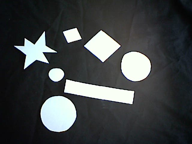
Zadani
Spocitejte kolik objektu urciteho typu se objevuje na obrazku z webkamery. Rozeznavame nasledujici typy objektu:
- Kolecko
- Ctvrec
- Obdelnik
- Hvezda
Trenovaci data naleznete zde
- Odevzdejte skript ve formátu
.ipynbnebo.py - V názvu souboru uveďte své jméno
- Jako parametr nechť je URL k obrázku
In [ ]:
Classifiers
In [1]:
train_target = [1,1,1,2,2,2,3,3,3]
In [ ]:
# Features - příznaky
train_data = np.zeros([9,2])
print(train_data)
for objnumber in range(1, len(props)):
    train_data[objnumber - 1, 0] = props[objnumber].area
    train_data[objnumber - 1, 1] = props[objnumber].perimeter
print(train_data)
In [ ]:
# Training
from sklearn import svm
svc = svm.SVC()
svc.fit(train_data, train_target)
In [ ]:
# Testing
y_pred = svc.predict(test_data)
y_pred
In [ ]:
y_pred = svc.predict([[300, 7800]])
y_pred